An Introduction to Statistical Learning:

8.4 Exercises

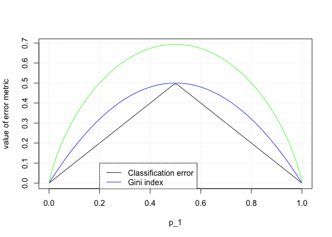
Exercise 3

p1 <- seq(0 + 1e-06, 1 - 1e-06, length.out = 100)
p2 <- 1 - p1

# The missclassification error-rate:
E <- 1 - apply(rbind(p1, p2), 2, max)

# The Gini index:
G <- p1 * (1 - p1) + p2 * (1 - p2)

# The cross-entropy:
D <- -(p1 * log(p1) + p2 * log(p2))

plot(p1, E, type = "l", col = "black", xlab = "p_1", ylab = "value of error metric", ylim = c(min(c(E, G, D)), max(E, G, D)))
lines(p1, G, col = "blue")
lines(p1, D, col = "green")
legend(0.2, 0.1, c("Classification error", "Gini index", "Cross entropy"), col = c("black", "blue", "green"), lty = c(1, 1))
grid()

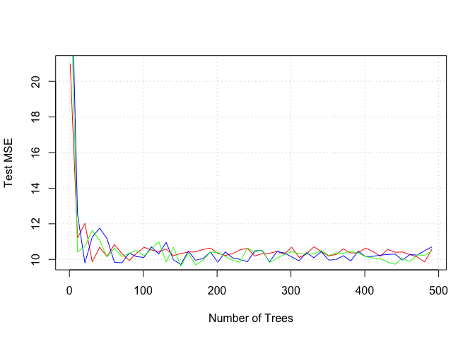
Exercise 7

library(MASS)
library(randomForest)

## randomForest 4.6-10
## Type rfNews() to see new features/changes/bug fixes.

set.seed(0)

n <- nrow(Boston)
p <- ncol(Boston) - 1  # one column is the response we are trying to model i.e. 'medv' 

train <- sample(1:n, n/2)
test <- (1:n)[-train]

ntree_to_test <- seq(from = 1, to = 500, by = 10)

# For a number of mtry values and a number of trees look at the test error rate:

# For mtry == p:
mse.bag <- rep(NA, length(ntree_to_test))
for (nti in 1:length(ntree_to_test)) {
    nt <- ntree_to_test[nti]

    # Grow a tree with 'nt' trees:
    boston.bag <- randomForest(medv ~ ., data = Boston, mtry = p, ntree = nt, importance = TRUE, subset = train)

    # Make predictions with this tree on the test dataset:
    y_hat <- predict(boston.bag, newdata = Boston[test, ])

    mse.bag[nti] <- mean((Boston[test, ]$medv - y_hat)^2)
}

# For mtry=p/2:
mse.p_over_two <- rep(NA, length(ntree_to_test))
for (nti in 1:length(ntree_to_test)) {
    nt <- ntree_to_test[nti]

    # Grow a tree with 'nt' trees:
    boston.bag <- randomForest(medv ~ ., data = Boston, mtry = p/2, ntree = nt, importance = TRUE, subset = train)

    # Make predictions with this tree on the test dataset:
    y_hat <- predict(boston.bag, newdata = Boston[test, ])

    mse.p_over_two[nti] <- mean((Boston[test, ]$medv - y_hat)^2)
}


# Run random forest with mtry=sqrt(p) and test on test set
mse.sqrt_p <- rep(NA, length(ntree_to_test))
for (nti in 1:length(ntree_to_test)) {
    nt <- ntree_to_test[nti]

    # Grow a tree with 'nt' trees:
    boston.bag <- randomForest(medv ~ ., data = Boston, mtry = p/2, ntree = nt, importance = TRUE, subset = train)

    # Make predictions with this tree on the test dataset:
    y_hat <- predict(boston.bag, newdata = Boston[test, ])

    mse.sqrt_p[nti] <- mean((Boston[test, ]$medv - y_hat)^2)
}

plot(ntree_to_test, mse.bag, xlab = "Number of Trees", ylab = "Test MSE", col = "red", type = "l")
lines(ntree_to_test, mse.p_over_two, xlab = "Number of Trees", ylab = "Test MSE", col = "blue", type = "l")
lines(ntree_to_test, mse.sqrt_p, xlab = "Number of Trees", ylab = "Test MSE", col = "green", type = "l")
grid()

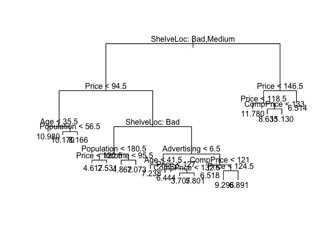
Exercise 8

library(tree)
library(ISLR)
attach(Carseats)

set.seed(0)

n <- nrow(Carseats)
p <- ncol(Carseats) - 1  # remove the column we seek to predict i.e. Sales

# Part (a):
train <- sample(1:n, n/2)
test <- (1:n)[-train]

# Part (b):
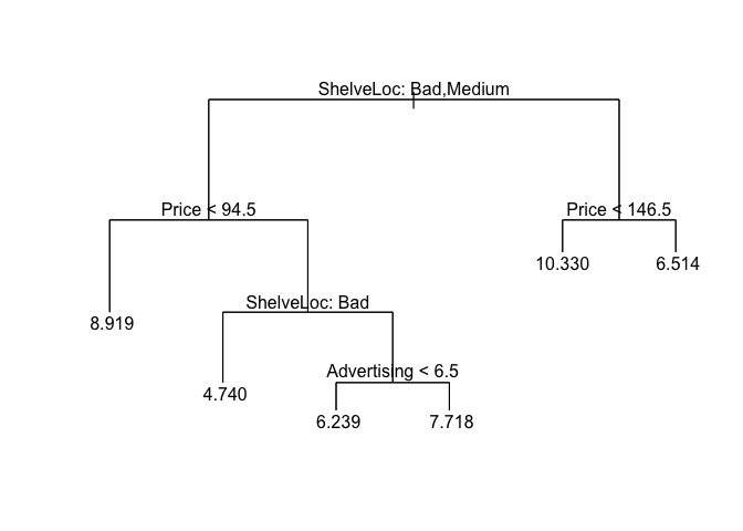
rtree.carseats <- tree(Sales ~ ., data = Carseats[train, ])
summary(rtree.carseats)

## 
## Regression tree:
## tree(formula = Sales ~ ., data = Carseats[train, ])
## Variables actually used in tree construction:
## [1] "ShelveLoc"   "Price"       "Age"         "Population"  "Income"     
## [6] "Advertising" "CompPrice"  
## Number of terminal nodes:  18 
## Residual mean deviance:  1.828 = 332.6 / 182 
## Distribution of residuals:
##     Min.  1st Qu.   Median     Mean  3rd Qu.     Max. 
## -3.47100 -0.85760  0.01643  0.00000  0.96960  3.09800

plot(rtree.carseats)
text(rtree.carseats, pretty = 0)

print(rtree.carseats)

## node), split, n, deviance, yval
##       * denotes terminal node
## 
##   1) root 200 1282.000  7.275  
##     2) ShelveLoc: Bad,Medium 168  884.600  6.807  
##       4) Price < 94.5 32   94.160  8.919  
##         8) Age < 35.5 5   12.750 10.980 *
##         9) Age > 35.5 27   56.200  8.537  
##          18) Population < 56.5 5   10.500 10.170 *
##          19) Population > 56.5 22   29.300  8.166 *
##       5) Price > 94.5 136  614.000  6.309  
##        10) ShelveLoc: Bad 39  138.300  4.740  
##          20) Population < 180.5 14   32.200  3.574  
##            40) Price < 120.5 7    4.681  4.617 *
##            41) Price > 120.5 7   12.300  2.531 *
##          21) Population > 180.5 25   76.380  5.392  
##            42) Income < 95.5 19   26.870  4.862 *
##            43) Income > 95.5 6   27.200  7.073 *
##        11) ShelveLoc: Medium 97  341.000  6.941  
##          22) Advertising < 6.5 51  129.300  6.239  
##            44) Age < 41.5 14   16.590  7.238 *
##            45) Age > 41.5 37   93.490  5.861  
##              90) Price < 127 23   34.700  6.444 *
##              91) Price > 127 14   38.140  4.904  
##               182) CompPrice < 132.5 6    5.325  3.707 *
##               183) CompPrice > 132.5 8   17.770  5.801 *
##          23) Advertising > 6.5 46  158.800  7.718  
##            46) CompPrice < 121 14   27.200  6.518 *
##            47) CompPrice > 121 32  102.500  8.244  
##              94) Price < 124.5 18   25.190  9.296 *
##              95) Price > 124.5 14   31.840  6.891 *
##     3) ShelveLoc: Good 32  167.000  9.735  
##       6) Price < 146.5 27   92.560 10.330  
##        12) Price < 118.5 9   11.530 11.780 *
##        13) Price > 118.5 18   52.580  9.606  
##          26) CompPrice < 133 11   11.550  8.635 *
##          27) CompPrice > 133 7   14.360 11.130 *
##       7) Price > 146.5 5   12.960  6.514 *

y_hat <- predict(rtree.carseats, newdata = Carseats[test, ])
test.MSE <- mean((y_hat - Carseats[test, ]$Sales)^2)
print(test.MSE)

## [1] 4.477452

# Part (c): Use cross-validation to determine the optimal of tree complexity:
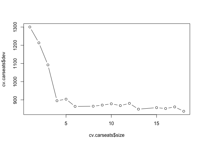
cv.carseats <- cv.tree(rtree.carseats)
names(cv.carseats)

## [1] "size"   "dev"    "k"      "method"

print(cv.carseats)

## $size
##  [1] 18 17 16 15 13 12 11 10  9  8  6  5  4  3  2  1
## 
## $dev
##  [1]  837.3778  861.1636  852.3690  857.1999  848.9026  880.5561  868.5359
##  [8]  878.2036  871.2037  865.0657  863.9906  903.7486  895.1975 1092.0162
## [15] 1213.2771 1300.3878
## 
## $k
##  [1]      -Inf  15.04210  15.22571  16.39571  19.95047  22.30687  25.21139
##  [8]  26.66949  28.45630  29.66510  37.26307  52.93732  61.48054 134.73740
## [15] 176.45091 230.50903
## 
## $method
## [1] "deviance"
## 
## attr(,"class")
## [1] "prune"         "tree.sequence"

plot(cv.carseats$size, cv.carseats$dev, type = "b")  # plot the tree size

# Pick the size of the tree you want to prune to: It looks like k=6 is the smallest tree with an error close to the minimum.

prune.carseats <- prune.tree(rtree.carseats, best = 6)

plot(prune.carseats)
text(prune.carseats, pretty = 0)

# Predict the MSE using this tree:
y_hat <- predict(prune.carseats, newdata = Carseats[test, ])
prune.MSE <- mean((y_hat - Carseats[test, ]$Sales)^2)
print(prune.MSE)

## [1] 5.208115

# Part (d): Use bagging
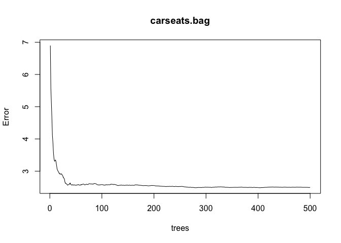
carseats.bag <- randomForest(Sales ~ ., data = Carseats, mtry = p, ntree = 500, importance = TRUE, subset = train)
y_hat <- predict(carseats.bag, newdata = Carseats[test, ])
mse.bag <- mean((Carseats[test, ]$Sales - y_hat)^2)
print(mse.bag)

## [1] 2.932783

plot(carseats.bag)

ibag <- importance(carseats.bag)
print(ibag[order(ibag[, 1]), ])

##                %IncMSE IncNodePurity
## Population  -1.9984333     54.142939
## Urban       -0.6258907      7.397644
## Income       0.9075028     60.629023
## Education    2.7940569     42.414542
## US           5.2112303     10.687375
## Advertising 11.9998791     86.644936
## Age         14.5356992    118.623427
## CompPrice   21.4674924    127.767968
## ShelveLoc   49.7905463    348.452887
## Price       57.4299058    380.441111

# Part (e): Use random forests
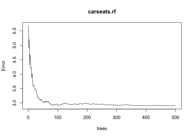
carseats.rf <- randomForest(Sales ~ ., data = Carseats, ntree = 500, mtry = p/3, importance = TRUE, subset = train)
y_hat <- predict(carseats.rf, newdata = Carseats[test, ])
mse.rf <- mean((Carseats[test, ]$Sales - y_hat)^2)
print(mse.rf)

## [1] 3.673223

plot(carseats.rf)

irf <- importance(carseats.rf)
print(irf[order(irf[, 1]), ])

##                %IncMSE IncNodePurity
## Population  -3.3907326      90.58748
## Urban       -1.2095544      10.28038
## Education    0.7890977      60.82180
## Income       1.9668734      93.81426
## US           2.1490545      15.16011
## CompPrice   10.8896740     114.42913
## Age         12.2675136     150.19842
## Advertising 13.9004159     114.95596
## ShelveLoc   33.1071231     259.08665
## Price       36.7085556     298.84473

Exercise 9

set.seed(0)

n <- nrow(OJ)
p <- ncol(OJ) - 1  # remove the response Purchase

# Part (a):
train <- sample(1:n, 800)
test <- (1:n)[-train]

# Part (b):
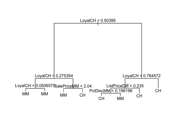
tree.OJ <- tree(Purchase ~ ., data = OJ[train, ])
summary(tree.OJ)

## 
## Classification tree:
## tree(formula = Purchase ~ ., data = OJ[train, ])
## Variables actually used in tree construction:
## [1] "LoyalCH"       "SalePriceMM"   "ListPriceDiff" "PctDiscMM"    
## Number of terminal nodes:  8 
## Residual mean deviance:  0.7414 = 587.2 / 792 
## Misclassification error rate: 0.1575 = 126 / 800

print(tree.OJ)

## node), split, n, deviance, yval, (yprob)
##       * denotes terminal node
## 
##  1) root 800 1067.00 CH ( 0.61375 0.38625 )  
##    2) LoyalCH < 0.50395 346  412.40 MM ( 0.28324 0.71676 )  
##      4) LoyalCH < 0.275354 160  104.00 MM ( 0.10000 0.90000 )  
##        8) LoyalCH < 0.0506575 58    0.00 MM ( 0.00000 1.00000 ) *
##        9) LoyalCH > 0.0506575 102   88.62 MM ( 0.15686 0.84314 ) *
##      5) LoyalCH > 0.275354 186  255.20 MM ( 0.44086 0.55914 )  
##       10) SalePriceMM < 2.04 99  117.90 MM ( 0.28283 0.71717 ) *
##       11) SalePriceMM > 2.04 87  115.50 CH ( 0.62069 0.37931 ) *
##    3) LoyalCH > 0.50395 454  358.30 CH ( 0.86564 0.13436 )  
##      6) LoyalCH < 0.764572 182  214.00 CH ( 0.72527 0.27473 )  
##       12) ListPriceDiff < 0.235 75  103.90 CH ( 0.52000 0.48000 )  
##         24) PctDiscMM < 0.196196 59   77.94 CH ( 0.62712 0.37288 ) *
##         25) PctDiscMM > 0.196196 16   12.06 MM ( 0.12500 0.87500 ) *
##       13) ListPriceDiff > 0.235 107   83.03 CH ( 0.86916 0.13084 ) *
##      7) LoyalCH > 0.764572 272   92.12 CH ( 0.95956 0.04044 ) *

plot(tree.OJ)
text(tree.OJ, pretty = 0)

y_hat <- predict(tree.OJ, newdata = OJ[test, ], type = "class")  # gives classification labels
CT <- table(y_hat, OJ[test, ]$Purchase)
print(CT)

##      
## y_hat  CH  MM
##    CH 142  27
##    MM  20  81

print("original tree: classificaion error rate on the test dataset:")

## [1] "original tree: classificaion error rate on the test dataset:"

print((CT[1, 2] + CT[2, 1])/sum(CT))

## [1] 0.1740741

# Part (c): Use cross-validation to determine the optimal of tree complexity:
cv.OJ <- cv.tree(tree.OJ)

plot(cv.OJ$size, cv.OJ$dev, type = "b")

# Pick the size of the tree you want to prune to:

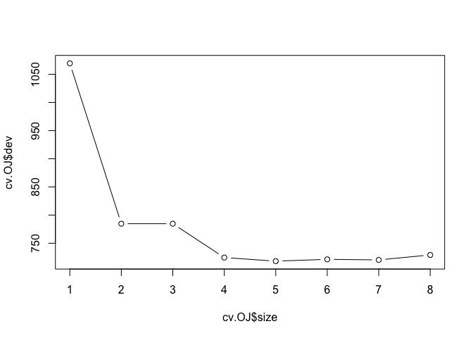
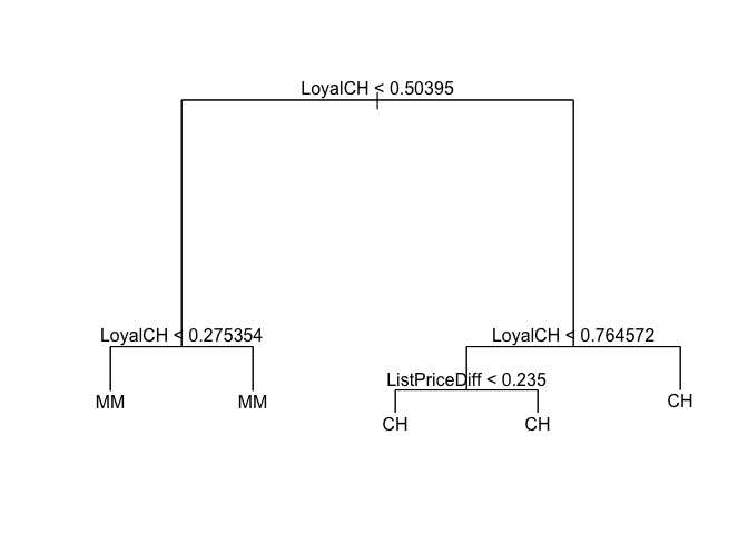
prune.OJ <- prune.tree(tree.OJ, best = 5)

plot(prune.OJ)
text(prune.OJ, pretty = 0)

# Compute training error rates:
y_hat <- predict(prune.OJ, newdata = OJ[train, ], type = "class")
CT <- table(y_hat, OJ[train, ]$Purchase)
print("pruned tree: classificaion error rate on the training dataset:")

## [1] "pruned tree: classificaion error rate on the training dataset:"

print((CT[1, 2] + CT[2, 1])/sum(CT))

## [1] 0.19875

# Compute testing error rates:
y_hat <- predict(prune.OJ, newdata = OJ[test, ], type = "class")
CT <- table(y_hat, OJ[test, ]$Purchase)
print("pruned tree: classificaion error rate on the test dataset:")

## [1] "pruned tree: classificaion error rate on the test dataset:"

print((CT[1, 2] + CT[2, 1])/sum(CT))

## [1] 0.2037037

Exercise 10

library(gbm)

## Loading required package: survival
## Loading required package: lattice
## Loading required package: splines
## Loading required package: parallel
## Loaded gbm 2.1.1

library(glmnet)

## Loading required package: Matrix
## Loading required package: foreach
## Loaded glmnet 2.0-2

set.seed(0)

Hitters <- na.omit(Hitters)
Hitters$Salary <- log(Hitters$Salary)

n <- nrow(Hitters)
p <- ncol(Hitters) - 1  # one column is the response we are trying to model i.e. 'Salary' 

train <- 1:200
test <- 201:n

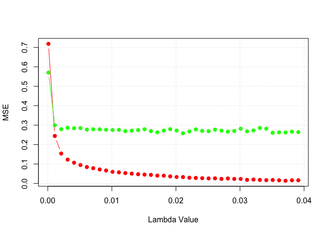
lambda_set <- seq(1e-04, 0.04, by = 0.001)

# 
training_set_mse <- rep(NA, length(lambda_set))
test_set_mse <- rep(NA, length(lambda_set))
for (lmi in 1:length(lambda_set)) {
    lm <- lambda_set[lmi]

    boost.hitters <- gbm(Salary ~ ., data = Hitters[train, ], distribution = "gaussian", n.trees = 1000, interaction.depth = 4, shrinkage = lm)

    y_hat <- predict(boost.hitters, newdata = Hitters[train, ], n.trees = 1000)
    training_set_mse[lmi] <- mean((y_hat - Hitters[train, ]$Salary)^2)

    y_hat <- predict(boost.hitters, newdata = Hitters[test, ], n.trees = 1000)
    test_set_mse[lmi] <- mean((y_hat - Hitters[test, ]$Salary)^2)
}

plot(lambda_set, training_set_mse, type = "b", pch = 19, col = "red", xlab = "Lambda Value", ylab = "MSE")
lines(lambda_set, test_set_mse, type = "b", pch = 19, col = "green", xlab = "Lambda Value", ylab = "Test Set MSE")
grid()

# Looks like the test MSE results are insensitive to the exact value of lambda as long as its small enough:
lm <- 0.01
boost.hitters <- gbm(Salary ~ ., data = Hitters[train, ], distribution = "gaussian", n.trees = 1000, interaction.depth = 4, shrinkage = lm)
y_hat <- predict(boost.hitters, newdata = Hitters[test, ], n.trees = 1000)
print("regression boosting test MSE:")

## [1] "regression boosting test MSE:"

print(mean((y_hat - Hitters[test, ]$Salary)^2))

## [1] 0.2756909

# Try linear regression:
m <- lm(Salary ~ ., data = Hitters[train, ])
y_hat <- predict(m, newdata = Hitters[test, ])
print("linear regression test MSE:")

## [1] "linear regression test MSE:"

print(mean((y_hat - Hitters[test, ]$Salary)^2))

## [1] 0.4917959

# Try the lasso:
MM <- model.matrix(Salary ~ ., data = Hitters[train, ])
cv.out <- cv.glmnet(MM, Hitters[train, ]$Salary, alpha = 1)
bestlam <- cv.out$lambda.1se
print("lasso CV best value of lambda (one standard error)")

## [1] "lasso CV best value of lambda (one standard error)"

print(bestlam)

## [1] 0.1571939

lasso.mod <- glmnet(MM, Hitters[train, ]$Salary, alpha = 1)

MM_test <- model.matrix(Salary ~ ., data = Hitters[test, ])
y_hat <- predict(lasso.mod, s = bestlam, newx = MM_test)
print("lasso regression test MSE:")

## [1] "lasso regression test MSE:"

print(mean((y_hat - Hitters[test, ]$Salary)^2))

## [1] 0.4382486

# Try ridge regression:
cv.out <- cv.glmnet(MM, Hitters[train, ]$Salary, alpha = 0)
plot(cv.out)

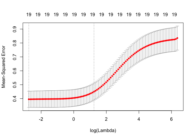
bestlam <- cv.out$lambda.1se
print("ridge CV best value of lambda (one standard error)")

## [1] "ridge CV best value of lambda (one standard error)"

print(bestlam)

## [1] 3.46633

ridge.mod <- glmnet(MM, Hitters[train, ]$Salary, alpha = 0)
Y_hat <- predict(ridge.mod, s = bestlam, newx = MM_test)
print("ridge regression test MSE:")

## [1] "ridge regression test MSE:"

print(mean((y_hat - Hitters[test, ]$Salary)^2))

## [1] 0.4382486

# What are the most important variables:
summary(boost.hitters)

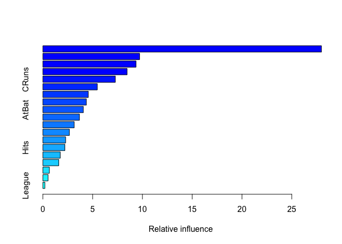
##                 var    rel.inf
## CAtBat       CAtBat 27.9843348
## CHits         CHits  9.7163571
## CRBI           CRBI  9.3564948
## CWalks       CWalks  8.4641693
## CRuns         CRuns  7.2820304
## Years         Years  5.4674280
## PutOuts     PutOuts  4.5604591
## Walks         Walks  4.3724216
## AtBat         AtBat  4.0692012
## CHmRun       CHmRun  3.6759612
## Assists     Assists  3.1511172
## RBI             RBI  2.6630040
## Errors       Errors  2.2909979
## Hits           Hits  2.2133744
## HmRun         HmRun  1.7480868
## Runs           Runs  1.5973072
## NewLeague NewLeague  0.6577638
## Division   Division  0.5252455
## League       League  0.2042459

# Try randomForests on the Hitters dataset (not asked for in the problem statement):
rf.hitters <- randomForest(Salary ~ ., data = Hitters, mtry = p/3, ntree = 1000, importance = TRUE, subset = train)
y_hat <- predict(rf.hitters, newdata = Hitters[test, ])
mse.rf <- mean((Hitters[test, ]$Salary - y_hat)^2)
print("randomForest test MSE:")

## [1] "randomForest test MSE:"

print(mse.rf)

## [1] 0.2171106

# Try BAGGING on the Hitters dataset:
bag.hitters <- randomForest(Salary ~ ., data = Hitters, mtry = p, ntree = 1000, importance = TRUE, subset = train)
y_hat <- predict(bag.hitters, newdata = Hitters[test, ])
mse.bag <- mean((Hitters[test, ]$Salary - y_hat)^2)
print("Bagging test MSE:")

## [1] "Bagging test MSE:"

print(mse.bag)

## [1] 0.2342413

Exercise 11

set.seed(0)

Caravan <- na.omit(Caravan)

n <- nrow(Caravan)
p <- ncol(Caravan) - 1  # one column is the response we are trying to model i.e. 'Purchase' 

train <- 1:1000
test <- 1001:n

# Transform the response 'Purchase' to be in [0,1] as required by gbm:
PurchaseBinary <- rep(0, n)
PurchaseBinary[Caravan$Purchase == "Yes"] <- 1
Caravan$Purchase <- PurchaseBinary

# Some variables seem to be very noninformative (have zero variance as reported by gbm):
Caravan$PVRAAUT <- NULL
Caravan$AVRAAUT <- NULL

# Train a gbm:
lm <- 0.01
boost.caravan <- gbm(Purchase ~ ., data = Caravan[train, ], distribution = "bernoulli", n.trees = 1000, interaction.depth = 2, shrinkage = lm)
summary(boost.caravan)

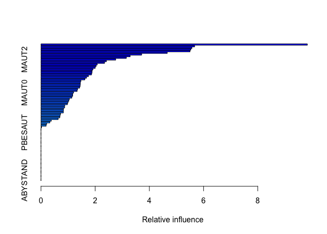
##               var    rel.inf
## PPERSAUT PPERSAUT 9.83047713
## MKOOPKLA MKOOPKLA 5.67101078
## MOPLHOOG MOPLHOOG 5.57015086
## PBRAND     PBRAND 5.53090647
## MGODGE     MGODGE 5.50146339
## MBERMIDD MBERMIDD 4.66053217
## MOSTYPE   MOSTYPE 3.71528842
## MINK3045 MINK3045 3.29167392
## MGODPR     MGODPR 3.15189659
## MAUT2       MAUT2 2.75860820
## MBERARBG MBERARBG 2.41585129
## ABRAND     ABRAND 2.34750399
## MSKC         MSKC 2.07742330
## MSKA         MSKA 2.03539655
## MAUT1       MAUT1 2.00290825
## MRELGE     MRELGE 1.91903070
## MSKB1       MSKB1 1.88713704
## PWAPART   PWAPART 1.88354710
## MFWEKIND MFWEKIND 1.86568208
## MGODOV     MGODOV 1.75362888
## MINK7512 MINK7512 1.68185238
## MFGEKIND MFGEKIND 1.62053883
## MBERHOOG MBERHOOG 1.47386158
## MBERARBO MBERARBO 1.45496977
## MINKM30   MINKM30 1.45332376
## MHKOOP     MHKOOP 1.44894919
## MGODRK     MGODRK 1.42859782
## MRELOV     MRELOV 1.35136073
## MINKGEM   MINKGEM 1.33514219
## MAUT0       MAUT0 1.20352717
## MZFONDS   MZFONDS 1.17292916
## MINK4575 MINK4575 1.16903944
## MOSHOOFD MOSHOOFD 1.13985697
## MHHUUR     MHHUUR 1.04951077
## MGEMLEEF MGEMLEEF 1.03005616
## APERSAUT APERSAUT 0.99864198
## MSKB2       MSKB2 0.97672510
## PBYSTAND PBYSTAND 0.87858256
## MOPLMIDD MOPLMIDD 0.87431940
## PMOTSCO   PMOTSCO 0.83289524
## MFALLEEN MFALLEEN 0.82850043
## MZPART     MZPART 0.82588303
## PLEVEN     PLEVEN 0.72568141
## MGEMOMV   MGEMOMV 0.70719044
## MSKD         MSKD 0.69605715
## MBERBOER MBERBOER 0.63402319
## MBERZELF MBERZELF 0.38036763
## MRELSA     MRELSA 0.32946406
## MINK123M MINK123M 0.21200829
## MOPLLAAG MOPLLAAG 0.19163868
## MAANTHUI MAANTHUI 0.02438834
## PWABEDR   PWABEDR 0.00000000
## PWALAND   PWALAND 0.00000000
## PBESAUT   PBESAUT 0.00000000
## PAANHANG PAANHANG 0.00000000
## PTRACTOR PTRACTOR 0.00000000
## PWERKT     PWERKT 0.00000000
## PBROM       PBROM 0.00000000
## PPERSONG PPERSONG 0.00000000
## PGEZONG   PGEZONG 0.00000000
## PWAOREG   PWAOREG 0.00000000
## PZEILPL   PZEILPL 0.00000000
## PPLEZIER PPLEZIER 0.00000000
## PFIETS     PFIETS 0.00000000
## PINBOED   PINBOED 0.00000000
## AWAPART   AWAPART 0.00000000
## AWABEDR   AWABEDR 0.00000000
## AWALAND   AWALAND 0.00000000
## ABESAUT   ABESAUT 0.00000000
## AMOTSCO   AMOTSCO 0.00000000
## AAANHANG AAANHANG 0.00000000
## ATRACTOR ATRACTOR 0.00000000
## AWERKT     AWERKT 0.00000000
## ABROM       ABROM 0.00000000
## ALEVEN     ALEVEN 0.00000000
## APERSONG APERSONG 0.00000000
## AGEZONG   AGEZONG 0.00000000
## AWAOREG   AWAOREG 0.00000000
## AZEILPL   AZEILPL 0.00000000
## APLEZIER APLEZIER 0.00000000
## AFIETS     AFIETS 0.00000000
## AINBOED   AINBOED 0.00000000
## ABYSTAND ABYSTAND 0.00000000

# Predict the testing error:
y_hat <- predict(boost.caravan, newdata = Caravan[test, ], n.trees = 1000)
p_hat <- exp(y_hat)/(1 + exp(y_hat))  # convert the logodd output into probabilities 

will_buy <- rep(0, length(test))
will_buy[p_hat > 0.2] <- 1

# Create a confusion matrix:
table(will_buy, Caravan[test, ]$Purchase)

##         
## will_buy    0    1
##        0 4357  253
##        1  176   36

# Train a logistic regression:
lr_model <- glm(Purchase ~ ., data = Caravan[train, ], family = "binomial")

## Warning: glm.fit: fitted probabilities numerically 0 or 1 occurred

y_hat <- predict(lr_model, newdata = Caravan[test, ])

## Warning in predict.lm(object, newdata, se.fit, scale = 1, type =
## ifelse(type == : prediction from a rank-deficient fit may be misleading

p_hat <- exp(y_hat)/(1 + exp(y_hat))  # convert the logodd output into probabilities 

will_buy <- rep(0, length(test))
will_buy[p_hat > 0.2] <- 1

# Create a confusion matrix:
table(will_buy, Caravan[test, ]$Purchase)

##         
## will_buy    0    1
##        0 4183  231
##        1  350   58