- Introduction
- 1. Chapter 2. Statistical Learning
- 2. Chapter 3. Linear Regression
- 3. Chapter 4. Classification
- 4. Chapter 5. Resampling Methods
- 5. Chapter 6. Linear Model Selection and Regularization
- 6. Chapter 7. Moving Beyond Linearity
- 7. Chapter 8. Tree-Based Methods
- 8. Chapter 9. Support Vector Machines
- 9. Chapter 10. Unsupervised Learning
- 10. References
- Published with GitBook
7.8 Lab: Non-linear Modeling
We begin by loading that ISLR package and attaching to the Wage dataset that we will be using throughtout this exercise.
library(ISLR)
attach(Wage)
7.8.1 Polynomial Regression and Step Functions
Let's fit a linear model to predict wage with a forth-degree polynomial using the poly()
fit <- lm(wage ~ poly(age, 4), data = Wage)
coef(summary(fit))
##                 Estimate Std. Error    t value     Pr(>|t|)
## (Intercept)    111.70361  0.7287409 153.283015 0.000000e+00
## poly(age, 4)1  447.06785 39.9147851  11.200558 1.484604e-28
## poly(age, 4)2 -478.31581 39.9147851 -11.983424 2.355831e-32
## poly(age, 4)3  125.52169 39.9147851   3.144742 1.678622e-03
## poly(age, 4)4  -77.91118 39.9147851  -1.951938 5.103865e-02
We can also obtain raw instead of orthogonal polynomials using the raw = TRUE argument to poly()
fit2 <- lm(wage ~ poly(age, 4, raw = T), data = Wage)
coef(summary(fit2))
##                             Estimate   Std. Error   t value     Pr(>|t|)
## (Intercept)            -1.841542e+02 6.004038e+01 -3.067172 0.0021802539
## poly(age, 4, raw = T)1  2.124552e+01 5.886748e+00  3.609042 0.0003123618
## poly(age, 4, raw = T)2 -5.638593e-01 2.061083e-01 -2.735743 0.0062606446
## poly(age, 4, raw = T)3  6.810688e-03 3.065931e-03  2.221409 0.0263977518
## poly(age, 4, raw = T)4 -3.203830e-05 1.641359e-05 -1.951938 0.0510386498
Finally, instead of using poly(), we can specify the polynomials directly in the formula as shown below.
fit2a <- lm(wage ~ age + I(age^2) + I(age^3) + I(age^4), data = Wage)
coef(fit2a)
##   (Intercept)           age      I(age^2)      I(age^3)      I(age^4)
## -1.841542e+02  2.124552e+01 -5.638593e-01  6.810688e-03 -3.203830e-05
A more compact version of the same example uses cbind() and eliminates the need to wrap each term in I().
fit2b <- lm(wage ~ cbind(age, age^2, age^3, age^4), data = Wage)
We can create an age grid for the targted values of the prediction and pass the grid to predict().
agelims <- range(age)
age.grid <- seq(from = agelims[1], to = agelims[2])
preds <- predict(fit, newdata = list(age = age.grid), se = TRUE)
se.bands <- cbind(preds$fit + 2 * preds$se.fit, preds$fit - 2 * preds$se.fit)
preds2 <- predict(fit2, newdata = list(age = age.grid), se = TRUE)
max(abs(preds$fit - preds2$fit))
## [1] 7.81597e-11
We can use anova() to compare five different models of linear fit.
fit.1 <- lm(wage ~ age, data = Wage)
fit.2 <- lm(wage ~ poly(age, 2), data = Wage)
fit.3 <- lm(wage ~ poly(age, 3), data = Wage)
fit.4 <- lm(wage ~ poly(age, 4), data = Wage)
fit.5 <- lm(wage ~ poly(age, 5), data = Wage)
anova(fit.1, fit.2, fit.3, fit.4, fit.5)
## Analysis of Variance Table
##
## Model 1: wage ~ age
## Model 2: wage ~ poly(age, 2)
## Model 3: wage ~ poly(age, 3)
## Model 4: wage ~ poly(age, 4)
## Model 5: wage ~ poly(age, 5)
##   Res.Df     RSS Df Sum of Sq        F    Pr(>F)
## 1   2998 5022216
## 2   2997 4793430  1    228786 143.5931 < 2.2e-16 ***
## 3   2996 4777674  1     15756   9.8888  0.001679 **
## 4   2995 4771604  1      6070   3.8098  0.051046 .
## 5   2994 4770322  1      1283   0.8050  0.369682
## ---
## Signif. codes:  0 '***' 0.001 '**' 0.01 '*' 0.05 '.' 0.1 ' ' 1
The same p-values can also be obtained from the coef() function.
coef(summary(fit.5))
##                 Estimate Std. Error     t value     Pr(>|t|)
## (Intercept)    111.70361  0.7287647 153.2780243 0.000000e+00
## poly(age, 5)1  447.06785 39.9160847  11.2001930 1.491111e-28
## poly(age, 5)2 -478.31581 39.9160847 -11.9830341 2.367734e-32
## poly(age, 5)3  125.52169 39.9160847   3.1446392 1.679213e-03
## poly(age, 5)4  -77.91118 39.9160847  -1.9518743 5.104623e-02
## poly(age, 5)5  -35.81289 39.9160847  -0.8972045 3.696820e-01
The anova() function can also compare the variances when other terms are included as predictors.
fit.1 <- lm(wage ~ education + age, data = Wage)
fit.2 <- lm(wage ~ education + poly(age, 2), data = Wage)
fit.3 <- lm(wage ~ education + poly(age, 3), data = Wage)
anova(fit.1, fit.2, fit.3)
## Analysis of Variance Table
##
## Model 1: wage ~ education + age
## Model 2: wage ~ education + poly(age, 2)
## Model 3: wage ~ education + poly(age, 3)
##   Res.Df     RSS Df Sum of Sq        F Pr(>F)
## 1   2994 3867992
## 2   2993 3725395  1    142597 114.6969 <2e-16 ***
## 3   2992 3719809  1      5587   4.4936 0.0341 *
## ---
## Signif. codes:  0 '***' 0.001 '**' 0.01 '*' 0.05 '.' 0.1 ' ' 1
With glm() we can also fit a polynomial logistic regression.
fit <- glm(I(wage > 250) ~ poly(age, 4), data = Wage, family = binomial)
And use the same method for making predictions using predict() as seen above.
preds <- predict(fit, newdata = list(age = age.grid), se = T)
pfit <- exp(preds$fit)/(1 + exp(preds$fit))
se.bands.logit <- cbind(preds$fit + 2 * preds$se.fit, preds$fit - 2 * preds$se.fit)
se.bands <- exp(se.bands.logit)/(1 + exp(se.bands.logit))
preds <- predict(fit, newdata = list(age = age.grid), type = "response", se = T)
We can plot these results with the plot() function as usual.
par(mfrow = c(1, 2), mar = c(4.5, 4.5, 1, 1), oma = c(0, 0, 4, 0))
plot(age, wage, xlim = agelims, cex = 0.5, col = "darkgrey")
title("Degree -4 Polynomial ", outer = T)
lines(age.grid, preds$fit, lwd = 2, col = "blue")
matlines(age.grid, se.bands, lwd = 1, col = "blue", lty = 3)

plot(age, I(wage > 250), xlim = agelims, type = "n", ylim = c(0, 0.2))
points(jitter(age), I((wage > 250)/5), cex = 0.5, pch = "|", col = " darkgrey ")
lines(age.grid, pfit, lwd = 2, col = "blue")
matlines(age.grid, se.bands, lwd = 1, col = "blue", lty = 3)
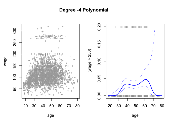
In the above plot, the jitter() function is used to prevent the same age obervations from overlapping each other.
The cut() functions creates cutpoints in the observations, which are then used as predictors for the linear model to fit a step function.
table(cut(age, 4))
##
## (17.9,33.5]   (33.5,49]   (49,64.5] (64.5,80.1]
##         750        1399         779          72
fit <- lm(wage ~ cut(age, 4), data = Wage)
coef(summary(fit))
##                         Estimate Std. Error   t value     Pr(>|t|)
## (Intercept)            94.158392   1.476069 63.789970 0.000000e+00
## cut(age, 4)(33.5,49]   24.053491   1.829431 13.148074 1.982315e-38
## cut(age, 4)(49,64.5]   23.664559   2.067958 11.443444 1.040750e-29
## cut(age, 4)(64.5,80.1]  7.640592   4.987424  1.531972 1.256350e-01
7.8.2 Splines
We use the splines package to run regression splines.
library(splines)
We first use bs() to generate a basis matrix for a polynomial spline and fit a model with knots at age 25, 40 and 60.
fit <- lm(wage ~ bs(age, knots = c(25, 40, 60)), data = Wage)
pred <- predict(fit, newdata = list(age = age.grid), se = T)
plot(age, wage, col = "gray")
lines(age.grid, pred$fit, lwd = 2)
lines(age.grid, pred$fit + 2 * pred$se, lty = "dashed")
lines(age.grid, pred$fit - 2 * pred$se, lty = "dashed")

Alternatively, the df() function can be used to produce a spline fit with knots at uniform intervals.
dim(bs(age, knots = c(25, 40, 60)))
## [1] 3000 6
dim(bs(age, df = 6))
## [1] 3000 6
attr(bs(age, df = 6), "knots")
##   25%   50%   75%
## 33.75 42.00 51.00
plot(age, wage, col = "gray")
fit2 <- lm(wage ~ ns(age, df = 4), data = Wage)
pred2 <- predict(fit2, newdata = list(age = age.grid), se = TRUE)
lines(age.grid, pred2$fit, col = "red", lwd = 2)
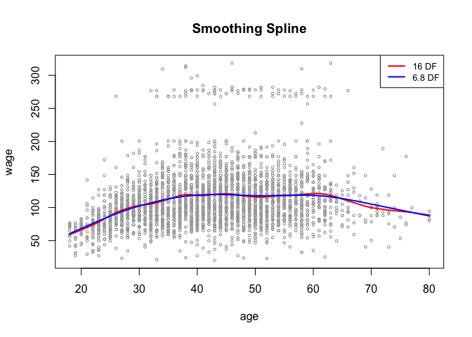
We can fit a smoothing spline using smooth.spline()
plot(age, wage, xlim = agelims, cex = 0.5, col = "darkgrey")
title(" Smoothing Spline ")
fit <- smooth.spline(age, wage, df = 16)
fit2 <- smooth.spline(age, wage, cv = TRUE)
## Warning in smooth.spline(age, wage, cv = TRUE): cross-validation with non-
## unique 'x' values seems doubtful
fit2$df
## [1] 6.794596
lines(fit, col = "red", lwd = 2)
lines(fit2, col = "blue", lwd = 2)
legend("topright", legend = c("16 DF", "6.8 DF"), col = c("red", "blue"), lty = 1, lwd = 2, cex = 0.8)
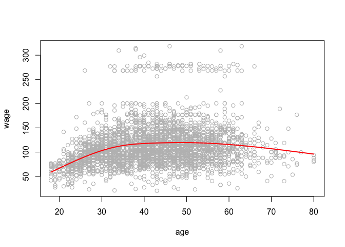
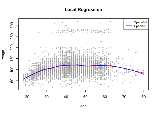
We can use loess() function for a local polynomial regression.
plot(age, wage, xlim = agelims, cex = 0.5, col = "darkgrey")
title(" Local Regression ")
fit <- loess(wage ~ age, span = 0.2, data = Wage)
fit2 <- loess(wage ~ age, span = 0.5, data = Wage)
lines(age.grid, predict(fit, data.frame(age = age.grid)), col = "red", lwd = 2)
lines(age.grid, predict(fit2, data.frame(age = age.grid)), col = "blue", lwd = 2)
legend("topright", legend = c("Span=0.2", "Span=0.5"), col = c("red", "blue"), lty = 1, lwd = 2, cex = 0.8)
7.8.3 GAMs
We can fit a GAM with lm() when an appropriate basis function can used.
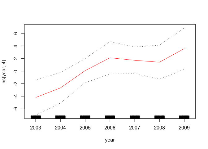
gam1 <- lm(wage ~ ns(year, 4) + ns(age, 5) + education, data = Wage)
However, the gam package offers a general solution to fitting GAMs and is especially useful when splines cannot be easily expressed in terms of basis functions.
library(gam)
## Loading required package: foreach
## Loaded gam 1.12
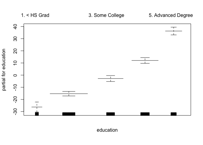
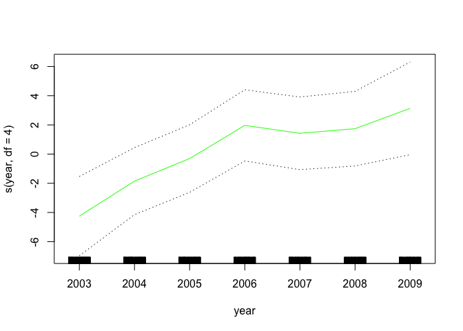
gam.m3 <- gam(wage ~ s(year, 4) + s(age, 5) + education, data = Wage)
The plot() function behaves the same way as it does with lm() and glm().
par(mfrow = c(1, 3))
plot(gam.m3, se = TRUE, col = "blue")
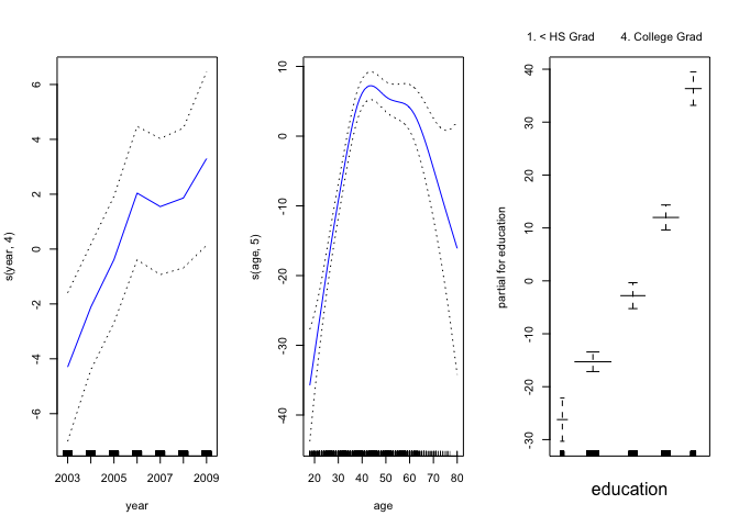
plot.gam(gam1, se = TRUE, col = "red")

We can use anova() to find the best performing model.
gam.m1 <- gam(wage ~ s(age, 5) + education, data = Wage)
gam.m2 <- gam(wage ~ year + s(age, 5) + education, data = Wage)
anova(gam.m1, gam.m2, gam.m3, test = "F")
## Analysis of Deviance Table
##
## Model 1: wage ~ s(age, 5) + education
## Model 2: wage ~ year + s(age, 5) + education
## Model 3: wage ~ s(year, 4) + s(age, 5) + education
##   Resid. Df Resid. Dev Df Deviance       F    Pr(>F)
## 1      2990    3711731
## 2      2989    3693842  1  17889.2 14.4771 0.0001447 ***
## 3      2986    3689770  3   4071.1  1.0982 0.3485661
## ---
## Signif. codes:  0 '***' 0.001 '**' 0.01 '*' 0.05 '.' 0.1 ' ' 1
And use summary() to generate a summary of the fitted model.
summary(gam.m3)
##
## Call: gam(formula = wage ~ s(year, 4) + s(age, 5) + education, data = Wage)
## Deviance Residuals:
##     Min      1Q  Median      3Q     Max
## -119.43  -19.70   -3.33   14.17  213.48
##
## (Dispersion Parameter for gaussian family taken to be 1235.69)
##
##     Null Deviance: 5222086 on 2999 degrees of freedom
## Residual Deviance: 3689770 on 2986 degrees of freedom
## AIC: 29887.75
##
## Number of Local Scoring Iterations: 2
##
## Anova for Parametric Effects
##              Df  Sum Sq Mean Sq F value    Pr(>F)
## s(year, 4)    1   27162   27162  21.981 2.877e-06 ***
## s(age, 5)     1  195338  195338 158.081 < 2.2e-16 ***
## education     4 1069726  267432 216.423 < 2.2e-16 ***
## Residuals  2986 3689770    1236
## ---
## Signif. codes:  0 '***' 0.001 '**' 0.01 '*' 0.05 '.' 0.1 ' ' 1
##
## Anova for Nonparametric Effects
##             Npar Df Npar F  Pr(F)
## (Intercept)
## s(year, 4)        3  1.086 0.3537
## s(age, 5)         4 32.380 <2e-16 ***
## education
## ---
## Signif. codes:  0 '***' 0.001 '**' 0.01 '*' 0.05 '.' 0.1 ' ' 1
We can make predictions using predict() just as we did with linear and logistic regressions.
preds <- predict(gam.m2, newdata = Wage)
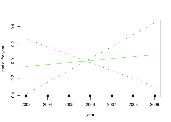
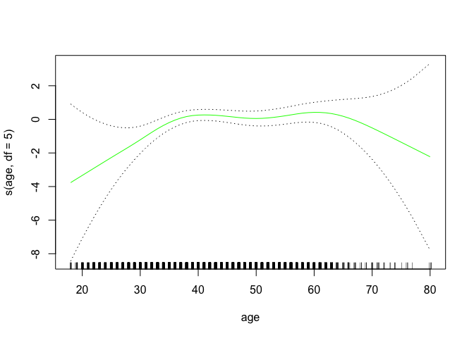
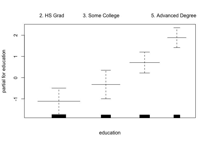
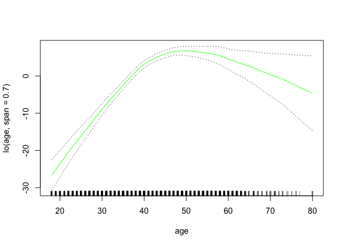
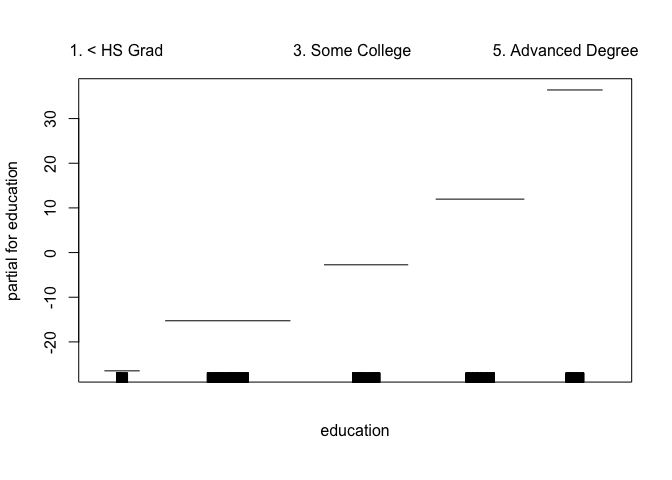
We can use a loess fit as a smoothing term in a GAM formula using the lo()
gam.lo <- gam(wage ~ s(year, df = 4) + lo(age, span = 0.7) + education, data = Wage)
plot.gam(gam.lo, se = TRUE, col = "green")

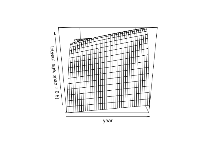
gam.lo.i <- gam(wage ~ lo(year, age, span = 0.5) + education, data = Wage)
The akima package can be used to plot tw-dimentional surface plots. Make sure the package is part of your R installation or install it with install.packages() if necessary.
library(akima)
plot(gam.lo.i)
The gam() function also allows fitting logistic regression GAM with the family = binomial argument.
gam.lr <- gam(I(wage > 250) ~ year + s(age, df = 5) + education, family = binomial, data = Wage)
par(mfrow = c(1, 3))
plot(gam.lr, se = T, col = "green")
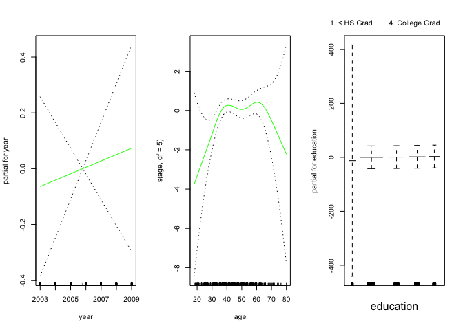
table(education, I(wage > 250))
##
## education            FALSE TRUE
##   1. < HS Grad         268    0
##   2. HS Grad           966    5
##   3. Some College      643    7
##   4. College Grad      663   22
##   5. Advanced Degree   381   45
gam.lr.s <- gam(I(wage > 250) ~ year + s(age, df = 5) + education, family = binomial, data = Wage, subset = (education != "1. < HS Grad"))
plot(gam.lr.s, se = T, col = "green")