- Introduction
- 1. Chapter 2. Statistical Learning
- 2. Chapter 3. Linear Regression
- 3. Chapter 4. Classification
- 4. Chapter 5. Resampling Methods
- 5. Chapter 6. Linear Model Selection and Regularization
- 6. Chapter 7. Moving Beyond Linearity
- 7. Chapter 8. Tree-Based Methods
- 8. Chapter 9. Support Vector Machines
- 9. Chapter 10. Unsupervised Learning
- 10. References
- Published with GitBook
6.5 Lab 1: Subset Selection Methods
6.5.1 Best Subset Selection
We start by loading the ISLR package and examining the Hitters dataset. We use the is.na() function and count the number of observations where the Salary variable is missing.
library(ISLR)
head(Hitters)
##                   AtBat Hits HmRun Runs RBI Walks Years CAtBat CHits
## -Andy Allanson      293   66     1   30  29    14     1    293    66
## -Alan Ashby         315   81     7   24  38    39    14   3449   835
## -Alvin Davis        479  130    18   66  72    76     3   1624   457
## -Andre Dawson       496  141    20   65  78    37    11   5628  1575
## -Andres Galarraga   321   87    10   39  42    30     2    396   101
## -Alfredo Griffin    594  169     4   74  51    35    11   4408  1133
##                   CHmRun CRuns CRBI CWalks League Division PutOuts Assists
## -Andy Allanson         1    30   29     14      A        E     446      33
## -Alan Ashby           69   321  414    375      N        W     632      43
## -Alvin Davis          63   224  266    263      A        W     880      82
## -Andre Dawson        225   828  838    354      N        E     200      11
## -Andres Galarraga     12    48   46     33      N        E     805      40
## -Alfredo Griffin      19   501  336    194      A        W     282     421
##                   Errors Salary NewLeague
## -Andy Allanson        20     NA         A
## -Alan Ashby           10  475.0         N
## -Alvin Davis          14  480.0         A
## -Andre Dawson          3  500.0         N
## -Andres Galarraga      4   91.5         N
## -Alfredo Griffin      25  750.0         A
names(Hitters)
##  [1] "AtBat"     "Hits"      "HmRun"     "Runs"      "RBI"
##  [6] "Walks"     "Years"     "CAtBat"    "CHits"     "CHmRun"
## [11] "CRuns"     "CRBI"      "CWalks"    "League"    "Division"
## [16] "PutOuts"   "Assists"   "Errors"    "Salary"    "NewLeague"
dim(Hitters)
## [1] 322 20
sum(is.na(Hitters$Salary))
## [1] 59
We can remove all observations with missing values with na.omit().
Hitters <- na.omit(Hitters)
dim(Hitters)
## [1] 263 20
sum(is.na(Hitters))
## [1] 0
We use the regsubsets() function to identify the best model based on subset selection quantified by the residual sum of squares (RSS) for each model.
library(leaps)
regfit.full <- regsubsets(Salary ~ ., Hitters)
summary(regfit.full)
## Subset selection object
## Call: regsubsets.formula(Salary ~ ., Hitters)
## 19 Variables  (and intercept)
##            Forced in Forced out
## AtBat          FALSE      FALSE
## Hits           FALSE      FALSE
## HmRun          FALSE      FALSE
## Runs           FALSE      FALSE
## RBI            FALSE      FALSE
## Walks          FALSE      FALSE
## Years          FALSE      FALSE
## CAtBat         FALSE      FALSE
## CHits          FALSE      FALSE
## CHmRun         FALSE      FALSE
## CRuns          FALSE      FALSE
## CRBI           FALSE      FALSE
## CWalks         FALSE      FALSE
## LeagueN        FALSE      FALSE
## DivisionW      FALSE      FALSE
## PutOuts        FALSE      FALSE
## Assists        FALSE      FALSE
## Errors         FALSE      FALSE
## NewLeagueN     FALSE      FALSE
## 1 subsets of each size up to 8
## Selection Algorithm: exhaustive
##          AtBat Hits HmRun Runs RBI Walks Years CAtBat CHits CHmRun CRuns
## 1  ( 1 ) " "   " "  " "   " "  " " " "   " "   " "    " "   " "    " "
## 2  ( 1 ) " "   "*"  " "   " "  " " " "   " "   " "    " "   " "    " "
## 3  ( 1 ) " "   "*"  " "   " "  " " " "   " "   " "    " "   " "    " "
## 4  ( 1 ) " "   "*"  " "   " "  " " " "   " "   " "    " "   " "    " "
## 5  ( 1 ) "*"   "*"  " "   " "  " " " "   " "   " "    " "   " "    " "
## 6  ( 1 ) "*"   "*"  " "   " "  " " "*"   " "   " "    " "   " "    " "
## 7  ( 1 ) " "   "*"  " "   " "  " " "*"   " "   "*"    "*"   "*"    " "
## 8  ( 1 ) "*"   "*"  " "   " "  " " "*"   " "   " "    " "   "*"    "*"
##          CRBI CWalks LeagueN DivisionW PutOuts Assists Errors NewLeagueN
## 1  ( 1 ) "*"  " "    " "     " "       " "     " "     " "    " "
## 2  ( 1 ) "*"  " "    " "     " "       " "     " "     " "    " "
## 3  ( 1 ) "*"  " "    " "     " "       "*"     " "     " "    " "
## 4  ( 1 ) "*"  " "    " "     "*"       "*"     " "     " "    " "
## 5  ( 1 ) "*"  " "    " "     "*"       "*"     " "     " "    " "
## 6  ( 1 ) "*"  " "    " "     "*"       "*"     " "     " "    " "
## 7  ( 1 ) " "  " "    " "     "*"       "*"     " "     " "    " "
## 8  ( 1 ) " "  "*"    " "     "*"       "*"     " "     " "    " "
The nvmax parameter can be use to control the number of variables in the model. The default used by regsubsets() is 8.
regfit.full <- regsubsets(Salary ~ ., data = Hitters, nvmax = 19)
reg.summary <- summary(regfit.full)
We can look at the components of the reg.summary variable using the names() function and examine the (R^2) statistic stored in rsq.
names(reg.summary)
## [1] "which" "rsq" "rss" "adjr2" "cp" "bic" "outmat" "obj"
reg.summary$rsq
##  [1] 0.3214501 0.4252237 0.4514294 0.4754067 0.4908036 0.5087146 0.5141227
##  [8] 0.5285569 0.5346124 0.5404950 0.5426153 0.5436302 0.5444570 0.5452164
## [15] 0.5454692 0.5457656 0.5459518 0.5460945 0.5461159
Next, we plot the RSS and adjusted (R^2) and add a point where (R^2) is at its maximum using the which.max() function.
par(mfrow = c(2, 2))
plot(reg.summary$rss, xlab = "Number of Variables", ylab = "RSS", type = "l")
plot(reg.summary$adjr2, xlab = "Number of Variables", ylab = "Adjusted RSq", type = "l")

adjr2.max <- which.max(reg.summary$adjr2)
points(adjr2.max, reg.summary$adjr2[adjr2.max], col = "red", cex = 2, pch = 20)

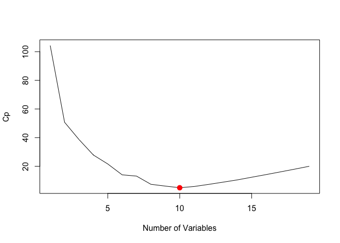
We can also plot the the (C_p) statistic and BIC and identify the minimum points for each statistic using the which.min() function.
plot(reg.summary$cp, xlab = "Number of Variables", ylab = "Cp", type = "l")
cp.min <- which.min(reg.summary$cp)
points(cp.min, reg.summary$cp[cp.min], col = "red", cex = 2, pch = 20)
bic.min <- which.min(reg.summary$bic)
plot(reg.summary$bic, xlab = "Number of Variables", ylab = "BIC", type = "l")
points(bic.min, reg.summary$bic[bic.min], col = "red", cex = 2, pch = 20)

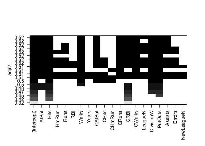
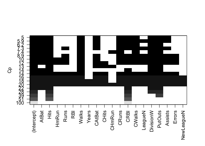
The estimated models from regsubsets() can be directly plotted to compare the differences based on the values of (R^2), adjusted (R^2), (C_p) and BIC statistics.
plot(regfit.full, scale = "r2")

plot(regfit.full, scale = "adjr2")
plot(regfit.full, scale = "Cp")
plot(regfit.full, scale = "bic")
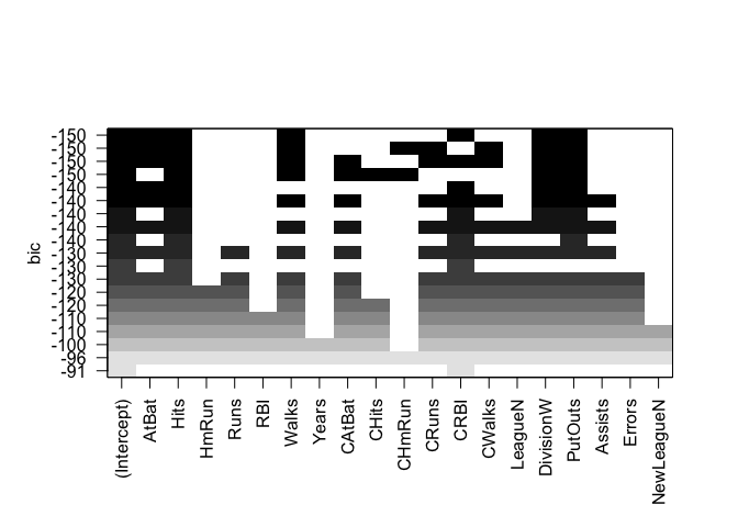
To show the coefficients associated with the model with the lowest BIC, we use the coef() function.
coef(regfit.full, bic.min)
##  (Intercept)        AtBat         Hits        Walks         CRBI
##   91.5117981   -1.8685892    7.6043976    3.6976468    0.6430169
##    DivisionW      PutOuts
## -122.9515338    0.2643076
6.5.2 Forward and Backward Stepwise Selection
The default method used by regsubsets() is exhaustive but we can change it to forward or backward and compare the results.
regfit.fwd <- regsubsets(Salary ~ ., data = Hitters, nvmax = 19, method = "forward")
summary(regfit.fwd)
## Subset selection object
## Call: regsubsets.formula(Salary ~ ., data = Hitters, nvmax = 19, method = "forward")
## 19 Variables  (and intercept)
##            Forced in Forced out
## AtBat          FALSE      FALSE
## Hits           FALSE      FALSE
## HmRun          FALSE      FALSE
## Runs           FALSE      FALSE
## RBI            FALSE      FALSE
## Walks          FALSE      FALSE
## Years          FALSE      FALSE
## CAtBat         FALSE      FALSE
## CHits          FALSE      FALSE
## CHmRun         FALSE      FALSE
## CRuns          FALSE      FALSE
## CRBI           FALSE      FALSE
## CWalks         FALSE      FALSE
## LeagueN        FALSE      FALSE
## DivisionW      FALSE      FALSE
## PutOuts        FALSE      FALSE
## Assists        FALSE      FALSE
## Errors         FALSE      FALSE
## NewLeagueN     FALSE      FALSE
## 1 subsets of each size up to 19
## Selection Algorithm: forward
##           AtBat Hits HmRun Runs RBI Walks Years CAtBat CHits CHmRun CRuns
## 1  ( 1 )  " "   " "  " "   " "  " " " "   " "   " "    " "   " "    " "
## 2  ( 1 )  " "   "*"  " "   " "  " " " "   " "   " "    " "   " "    " "
## 3  ( 1 )  " "   "*"  " "   " "  " " " "   " "   " "    " "   " "    " "
## 4  ( 1 )  " "   "*"  " "   " "  " " " "   " "   " "    " "   " "    " "
## 5  ( 1 )  "*"   "*"  " "   " "  " " " "   " "   " "    " "   " "    " "
## 6  ( 1 )  "*"   "*"  " "   " "  " " "*"   " "   " "    " "   " "    " "
## 7  ( 1 )  "*"   "*"  " "   " "  " " "*"   " "   " "    " "   " "    " "
## 8  ( 1 )  "*"   "*"  " "   " "  " " "*"   " "   " "    " "   " "    "*"
## 9  ( 1 )  "*"   "*"  " "   " "  " " "*"   " "   "*"    " "   " "    "*"
## 10  ( 1 ) "*"   "*"  " "   " "  " " "*"   " "   "*"    " "   " "    "*"
## 11  ( 1 ) "*"   "*"  " "   " "  " " "*"   " "   "*"    " "   " "    "*"
## 12  ( 1 ) "*"   "*"  " "   "*"  " " "*"   " "   "*"    " "   " "    "*"
## 13  ( 1 ) "*"   "*"  " "   "*"  " " "*"   " "   "*"    " "   " "    "*"
## 14  ( 1 ) "*"   "*"  "*"   "*"  " " "*"   " "   "*"    " "   " "    "*"
## 15  ( 1 ) "*"   "*"  "*"   "*"  " " "*"   " "   "*"    "*"   " "    "*"
## 16  ( 1 ) "*"   "*"  "*"   "*"  "*" "*"   " "   "*"    "*"   " "    "*"
## 17  ( 1 ) "*"   "*"  "*"   "*"  "*" "*"   " "   "*"    "*"   " "    "*"
## 18  ( 1 ) "*"   "*"  "*"   "*"  "*" "*"   "*"   "*"    "*"   " "    "*"
## 19  ( 1 ) "*"   "*"  "*"   "*"  "*" "*"   "*"   "*"    "*"   "*"    "*"
##           CRBI CWalks LeagueN DivisionW PutOuts Assists Errors NewLeagueN
## 1  ( 1 )  "*"  " "    " "     " "       " "     " "     " "    " "
## 2  ( 1 )  "*"  " "    " "     " "       " "     " "     " "    " "
## 3  ( 1 )  "*"  " "    " "     " "       "*"     " "     " "    " "
## 4  ( 1 )  "*"  " "    " "     "*"       "*"     " "     " "    " "
## 5  ( 1 )  "*"  " "    " "     "*"       "*"     " "     " "    " "
## 6  ( 1 )  "*"  " "    " "     "*"       "*"     " "     " "    " "
## 7  ( 1 )  "*"  "*"    " "     "*"       "*"     " "     " "    " "
## 8  ( 1 )  "*"  "*"    " "     "*"       "*"     " "     " "    " "
## 9  ( 1 )  "*"  "*"    " "     "*"       "*"     " "     " "    " "
## 10  ( 1 ) "*"  "*"    " "     "*"       "*"     "*"     " "    " "
## 11  ( 1 ) "*"  "*"    "*"     "*"       "*"     "*"     " "    " "
## 12  ( 1 ) "*"  "*"    "*"     "*"       "*"     "*"     " "    " "
## 13  ( 1 ) "*"  "*"    "*"     "*"       "*"     "*"     "*"    " "
## 14  ( 1 ) "*"  "*"    "*"     "*"       "*"     "*"     "*"    " "
## 15  ( 1 ) "*"  "*"    "*"     "*"       "*"     "*"     "*"    " "
## 16  ( 1 ) "*"  "*"    "*"     "*"       "*"     "*"     "*"    " "
## 17  ( 1 ) "*"  "*"    "*"     "*"       "*"     "*"     "*"    "*"
## 18  ( 1 ) "*"  "*"    "*"     "*"       "*"     "*"     "*"    "*"
## 19  ( 1 ) "*"  "*"    "*"     "*"       "*"     "*"     "*"    "*"
regfit.bwd <- regsubsets(Salary ~ ., data = Hitters, nvmax = 19, method = "backward")
summary(regfit.bwd)
## Subset selection object
## Call: regsubsets.formula(Salary ~ ., data = Hitters, nvmax = 19, method = "backward")
## 19 Variables  (and intercept)
##            Forced in Forced out
## AtBat          FALSE      FALSE
## Hits           FALSE      FALSE
## HmRun          FALSE      FALSE
## Runs           FALSE      FALSE
## RBI            FALSE      FALSE
## Walks          FALSE      FALSE
## Years          FALSE      FALSE
## CAtBat         FALSE      FALSE
## CHits          FALSE      FALSE
## CHmRun         FALSE      FALSE
## CRuns          FALSE      FALSE
## CRBI           FALSE      FALSE
## CWalks         FALSE      FALSE
## LeagueN        FALSE      FALSE
## DivisionW      FALSE      FALSE
## PutOuts        FALSE      FALSE
## Assists        FALSE      FALSE
## Errors         FALSE      FALSE
## NewLeagueN     FALSE      FALSE
## 1 subsets of each size up to 19
## Selection Algorithm: backward
##           AtBat Hits HmRun Runs RBI Walks Years CAtBat CHits CHmRun CRuns
## 1  ( 1 )  " "   " "  " "   " "  " " " "   " "   " "    " "   " "    "*"
## 2  ( 1 )  " "   "*"  " "   " "  " " " "   " "   " "    " "   " "    "*"
## 3  ( 1 )  " "   "*"  " "   " "  " " " "   " "   " "    " "   " "    "*"
## 4  ( 1 )  "*"   "*"  " "   " "  " " " "   " "   " "    " "   " "    "*"
## 5  ( 1 )  "*"   "*"  " "   " "  " " "*"   " "   " "    " "   " "    "*"
## 6  ( 1 )  "*"   "*"  " "   " "  " " "*"   " "   " "    " "   " "    "*"
## 7  ( 1 )  "*"   "*"  " "   " "  " " "*"   " "   " "    " "   " "    "*"
## 8  ( 1 )  "*"   "*"  " "   " "  " " "*"   " "   " "    " "   " "    "*"
## 9  ( 1 )  "*"   "*"  " "   " "  " " "*"   " "   "*"    " "   " "    "*"
## 10  ( 1 ) "*"   "*"  " "   " "  " " "*"   " "   "*"    " "   " "    "*"
## 11  ( 1 ) "*"   "*"  " "   " "  " " "*"   " "   "*"    " "   " "    "*"
## 12  ( 1 ) "*"   "*"  " "   "*"  " " "*"   " "   "*"    " "   " "    "*"
## 13  ( 1 ) "*"   "*"  " "   "*"  " " "*"   " "   "*"    " "   " "    "*"
## 14  ( 1 ) "*"   "*"  "*"   "*"  " " "*"   " "   "*"    " "   " "    "*"
## 15  ( 1 ) "*"   "*"  "*"   "*"  " " "*"   " "   "*"    "*"   " "    "*"
## 16  ( 1 ) "*"   "*"  "*"   "*"  "*" "*"   " "   "*"    "*"   " "    "*"
## 17  ( 1 ) "*"   "*"  "*"   "*"  "*" "*"   " "   "*"    "*"   " "    "*"
## 18  ( 1 ) "*"   "*"  "*"   "*"  "*" "*"   "*"   "*"    "*"   " "    "*"
## 19  ( 1 ) "*"   "*"  "*"   "*"  "*" "*"   "*"   "*"    "*"   "*"    "*"
##           CRBI CWalks LeagueN DivisionW PutOuts Assists Errors NewLeagueN
## 1  ( 1 )  " "  " "    " "     " "       " "     " "     " "    " "
## 2  ( 1 )  " "  " "    " "     " "       " "     " "     " "    " "
## 3  ( 1 )  " "  " "    " "     " "       "*"     " "     " "    " "
## 4  ( 1 )  " "  " "    " "     " "       "*"     " "     " "    " "
## 5  ( 1 )  " "  " "    " "     " "       "*"     " "     " "    " "
## 6  ( 1 )  " "  " "    " "     "*"       "*"     " "     " "    " "
## 7  ( 1 )  " "  "*"    " "     "*"       "*"     " "     " "    " "
## 8  ( 1 )  "*"  "*"    " "     "*"       "*"     " "     " "    " "
## 9  ( 1 )  "*"  "*"    " "     "*"       "*"     " "     " "    " "
## 10  ( 1 ) "*"  "*"    " "     "*"       "*"     "*"     " "    " "
## 11  ( 1 ) "*"  "*"    "*"     "*"       "*"     "*"     " "    " "
## 12  ( 1 ) "*"  "*"    "*"     "*"       "*"     "*"     " "    " "
## 13  ( 1 ) "*"  "*"    "*"     "*"       "*"     "*"     "*"    " "
## 14  ( 1 ) "*"  "*"    "*"     "*"       "*"     "*"     "*"    " "
## 15  ( 1 ) "*"  "*"    "*"     "*"       "*"     "*"     "*"    " "
## 16  ( 1 ) "*"  "*"    "*"     "*"       "*"     "*"     "*"    " "
## 17  ( 1 ) "*"  "*"    "*"     "*"       "*"     "*"     "*"    "*"
## 18  ( 1 ) "*"  "*"    "*"     "*"       "*"     "*"     "*"    "*"
## 19  ( 1 ) "*"  "*"    "*"     "*"       "*"     "*"     "*"    "*"
coef(regfit.full, 7)
##  (Intercept)         Hits        Walks       CAtBat        CHits
##   79.4509472    1.2833513    3.2274264   -0.3752350    1.4957073
##       CHmRun    DivisionW      PutOuts
##    1.4420538 -129.9866432    0.2366813
coef(regfit.fwd, 7)
##  (Intercept)        AtBat         Hits        Walks         CRBI
##  109.7873062   -1.9588851    7.4498772    4.9131401    0.8537622
##       CWalks    DivisionW      PutOuts
##   -0.3053070 -127.1223928    0.2533404
coef(regfit.bwd, 7)
##  (Intercept)        AtBat         Hits        Walks        CRuns
##  105.6487488   -1.9762838    6.7574914    6.0558691    1.1293095
##       CWalks    DivisionW      PutOuts
##   -0.7163346 -116.1692169    0.3028847
6.5.3 Choosing Among Models Using the Validation Set Approach and Cross-Validation
For validation set approach, we split the dataset into a training subset and a test subset. In order to ensure that the results are consistent over multiple iterations, we set the random seed with set.seed() before calling sample().
set.seed(1)
train <- sample(c(TRUE, FALSE), nrow(Hitters), rep = TRUE)
test <- (!train)
We use regsubsets() as we did in the last section, but limit the estimation to the training subset.
regfit.best <- regsubsets(Salary ~ ., data = Hitters[train, ], nvmax = 19)
We create a matrix from the test subset using model.matrix().
test.mat <- model.matrix(Salary ~ ., data = Hitters[test, ])
Next, we compute the validation error for each model.
val.errors <- rep(NA, 19)
for (i in 1:19) {
    coefi <- coef(regfit.best, id = i)
    pred <- test.mat[, names(coefi)] %*% coefi
    val.errors[i] <- mean((Hitters$Salary[test] - pred)^2)
}
We examine the validation error for each model and identify the best model with the lowest error.
val.errors
##  [1] 220968.0 169157.1 178518.2 163426.1 168418.1 171270.6 162377.1
##  [8] 157909.3 154055.7 148162.1 151156.4 151742.5 152214.5 157358.7
## [15] 158541.4 158743.3 159972.7 159859.8 160105.6
min.val.errors <- which.min(val.errors)
coef(regfit.best, min.val.errors)
## (Intercept)       AtBat        Hits       Walks      CAtBat       CHits
## -80.2751499  -1.4683816   7.1625314   3.6430345  -0.1855698   1.1053238
##      CHmRun      CWalks     LeagueN   DivisionW     PutOuts
##   1.3844863  -0.7483170  84.5576103 -53.0289658   0.2381662
We can combine these steps into a function that can be called repeatedly when running k-fold cross-validation.
predict.regsubsets <- function(object, newdata, id, ...) {
    form <- as.formula(object$call[[2]])
    mat <- model.matrix(form, newdata)
    coefi <- coef(object, id = id)
    xvars <- names(coefi)
    mat[, xvars] %*% coefi
}
As a final step, we run regsubsets() on the full dataset and examine the coefficients associated with the model that has the lower validation error.
regfit.best <- regsubsets(Salary ~ ., data = Hitters, nvmax = 19)
coef(regfit.best, min.val.errors)
##  (Intercept)        AtBat         Hits        Walks       CAtBat
##  162.5354420   -2.1686501    6.9180175    5.7732246   -0.1300798
##        CRuns         CRBI       CWalks    DivisionW      PutOuts
##    1.4082490    0.7743122   -0.8308264 -112.3800575    0.2973726
##      Assists
##    0.2831680
For cross-validation, we create the number of folds needed (10, in this case) and allocate a matrix for storing the results.
k <- 10
set.seed(1)
folds <- sample(1:k, nrow(Hitters), replace = TRUE)
cv.errors <- matrix(NA, k, 19, dimnames = list(NULL, paste(1:19)))
We then run through each fold in a for loop and predict the salary using our predict function. We then calculate the validation error for each fold and save them in the matrix created above.
for (j in 1:k) {
    best.fit <- regsubsets(Salary ~ ., data = Hitters[folds != j, ], nvmax = 19)
    for (i in 1:19) {
        pred <- predict(best.fit, Hitters[folds == j, ], id = i)
        cv.errors[j, i] <- mean((Hitters$Salary[folds == j] - pred)^2)
    }
}
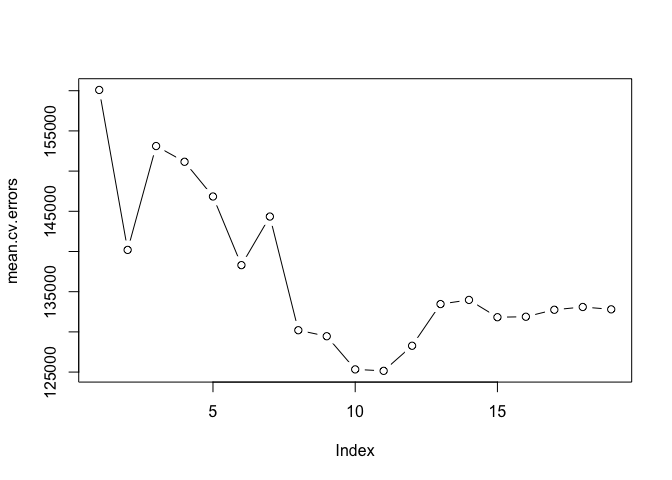
We calculate the mean error for all subsets by applying mean to each column using the apply() function
mean.cv.errors <- apply(cv.errors, 2, mean)
mean.cv.errors
##        1        2        3        4        5        6        7        8
## 160093.5 140196.8 153117.0 151159.3 146841.3 138302.6 144346.2 130207.7
##        9       10       11       12       13       14       15       16
## 129459.6 125334.7 125153.8 128273.5 133461.0 133974.6 131825.7 131882.8
##       17       18       19
## 132750.9 133096.2 132804.7
par(mfrow = c(1, 1))
plot(mean.cv.errors, type = "b")
Finally we run regsubsets() on the full dataset and show the coefficients for the best performing model.
reg.best <- regsubsets(Salary ~ ., data = Hitters, nvmax = 19)
coef(reg.best, which.min(mean.cv.errors))
##  (Intercept)        AtBat         Hits        Walks       CAtBat
##  135.7512195   -2.1277482    6.9236994    5.6202755   -0.1389914
##        CRuns         CRBI       CWalks      LeagueN    DivisionW
##    1.4553310    0.7852528   -0.8228559   43.1116152 -111.1460252
##      PutOuts      Assists
##    0.2894087    0.2688277
6.6 Lab 2: Ridge Regression and the Lasso
In order to run ridge regression, we first need to create a matrix from our dataset using the model.matrix() function.
x <- model.matrix(Salary ~ ., Hitters)[, -1]
y <- Hitters$Salary
6.6.1 Ridge Regression
The glmnet package provides functionality to fit ridge regression and lasso models. We load the package and call glmnet() to perform ridge regression.
library(glmnet)
## Loading required package: Matrix
## Loading required package: foreach
## Loaded glmnet 2.0-2
grid <- 10^seq(10, -2, length = 100)
ridge.mod <- glmnet(x, y, alpha = 0, lambda = grid)
dim(coef(ridge.mod))
## [1] 20 100
We can look at the coefficients at different values for (\lambda). Here we randomly choose two different values and notice that smaller values of (\lambda) result in larger coefficient estimates and vice-versa.
ridge.mod$lambda[50]
## [1] 11497.57
coef(ridge.mod)[, 50]
##   (Intercept)         AtBat          Hits         HmRun          Runs
## 407.356050200   0.036957182   0.138180344   0.524629976   0.230701523
##           RBI         Walks         Years        CAtBat         CHits
##   0.239841459   0.289618741   1.107702929   0.003131815   0.011653637
##        CHmRun         CRuns          CRBI        CWalks       LeagueN
##   0.087545670   0.023379882   0.024138320   0.025015421   0.085028114
##     DivisionW       PutOuts       Assists        Errors    NewLeagueN
##  -6.215440973   0.016482577   0.002612988  -0.020502690   0.301433531
sqrt(sum(coef(ridge.mod)[-1, 50]^2))
## [1] 6.360612
ridge.mod$lambda[60]
## [1] 705.4802
coef(ridge.mod)[, 60]
##  (Intercept)        AtBat         Hits        HmRun         Runs
##  54.32519950   0.11211115   0.65622409   1.17980910   0.93769713
##          RBI        Walks        Years       CAtBat        CHits
##   0.84718546   1.31987948   2.59640425   0.01083413   0.04674557
##       CHmRun        CRuns         CRBI       CWalks      LeagueN
##   0.33777318   0.09355528   0.09780402   0.07189612  13.68370191
##    DivisionW      PutOuts      Assists       Errors   NewLeagueN
## -54.65877750   0.11852289   0.01606037  -0.70358655   8.61181213
sqrt(sum(coef(ridge.mod)[-1, 60]^2))
## [1] 57.11001
We can get ridge regression coefficients for any value of (\lambda) using predict.
predict(ridge.mod, s = 50, type = "coefficients")[1:20, ]
##   (Intercept)         AtBat          Hits         HmRun          Runs
##  4.876610e+01 -3.580999e-01  1.969359e+00 -1.278248e+00  1.145892e+00
##           RBI         Walks         Years        CAtBat         CHits
##  8.038292e-01  2.716186e+00 -6.218319e+00  5.447837e-03  1.064895e-01
##        CHmRun         CRuns          CRBI        CWalks       LeagueN
##  6.244860e-01  2.214985e-01  2.186914e-01 -1.500245e-01  4.592589e+01
##     DivisionW       PutOuts       Assists        Errors    NewLeagueN
## -1.182011e+02  2.502322e-01  1.215665e-01 -3.278600e+00 -9.496680e+00
Next, we can cross-validation on ridge regression by first splitting the dataset into training and test subsets.
set.seed(1)
train <- sample(1:nrow(x), nrow(x)/2)
test <- (-train)
y.test <- y[test]
We estimate the parameters with glmnet() over the training set and predict the values on the test set to calculate the validation error.
ridge.mod <- glmnet(x[train, ], y[train], alpha = 0, lambda = grid, thresh = 1e-12)
ridge.pred <- predict(ridge.mod, s = 4, newx = x[test, ])
mean((ridge.pred - y.test)^2)
## [1] 101036.8
mean((mean(y[train]) - y.test)^2)
## [1] 193253.1
In the previous example, we used a value for (\lambda = 4) when evaluating the model on the test set. We can use a large value for (lamba) and see the difference in mean error.
ridge.pred <- predict(ridge.mod, s = 1e+10, newx = x[test, ])
mean((ridge.pred - y.test)^2)
## [1] 193253.1
We can also compare the results with a least squares model where (\lambda = 0).
ridge.pred <- predict(ridge.mod, s = 0, newx = x[test, ], exact = T)
mean((ridge.pred - y.test)^2)
## [1] 114783.1
lm(y ~ x, subset = train)
##
## Call:
## lm(formula = y ~ x, subset = train)
##
## Coefficients:
## (Intercept)       xAtBat        xHits       xHmRun        xRuns
##   299.42849     -2.54027      8.36682     11.64512     -9.09923
##        xRBI       xWalks       xYears      xCAtBat       xCHits
##     2.44105      9.23440    -22.93673     -0.18154     -0.11598
##     xCHmRun       xCRuns        xCRBI      xCWalks     xLeagueN
##    -1.33888      3.32838      0.07536     -1.07841     59.76065
##  xDivisionW     xPutOuts     xAssists      xErrors  xNewLeagueN
##   -98.86233      0.34087      0.34165     -0.64207     -0.67442
predict(ridge.mod, s = 0, exact = T, type = "coefficients")[1:20, ]
##  (Intercept)        AtBat         Hits        HmRun         Runs
## 299.42883596  -2.54014665   8.36611719  11.64400720  -9.09877719
##          RBI        Walks        Years       CAtBat        CHits
##   2.44152119   9.23403909 -22.93584442  -0.18160843  -0.11561496
##       CHmRun        CRuns         CRBI       CWalks      LeagueN
##  -1.33836534   3.32817777   0.07511771  -1.07828647  59.76529059
##    DivisionW      PutOuts      Assists       Errors   NewLeagueN
## -98.85996590   0.34086400   0.34165605  -0.64205839  -0.67606314
We can choose different values for (\lambda) by running cross-vaidation on ridge regression using cv.glmnet().
set.seed(1)
cv.out <- cv.glmnet(x[train, ], y[train], alpha = 0)
plot(cv.out)
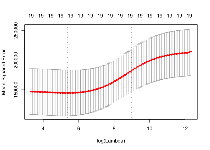
bestlam <- cv.out$lambda.min
bestlam
## [1] 211.7416
The best performing model is the one with (\lambda = 211.74).
ridge.pred <- predict(ridge.mod, s = bestlam, newx = x[test, ])
mean((ridge.pred - y.test)^2)
## [1] 96015.51
Finally, we run ridge regression on the full dataset and examine the coefficients for the model with the best MSE.
out <- glmnet(x, y, alpha = 0)
predict(out, type = "coefficients", s = bestlam)[1:20, ]
##  (Intercept)        AtBat         Hits        HmRun         Runs
##   9.88487157   0.03143991   1.00882875   0.13927624   1.11320781
##          RBI        Walks        Years       CAtBat        CHits
##   0.87318990   1.80410229   0.13074381   0.01113978   0.06489843
##       CHmRun        CRuns         CRBI       CWalks      LeagueN
##   0.45158546   0.12900049   0.13737712   0.02908572  27.18227535
##    DivisionW      PutOuts      Assists       Errors   NewLeagueN
## -91.63411299   0.19149252   0.04254536  -1.81244470   7.21208390
6.6.2 The Lasso
The lasso model can be estimated in the same way as ridge regression. The alpha = 1 parameter tells glmnet() to run lasso regression instead of ridge regression.
lasso.mod <- glmnet(x[train, ], y[train], alpha = 1, lambda = grid)
plot(lasso.mod)

Similarly, we can perform cross-validation using identical step as we did in the last exercise on ridge regression.
set.seed(1)
cv.out <- cv.glmnet(x[train, ], y[train], alpha = 1)
plot(cv.out)
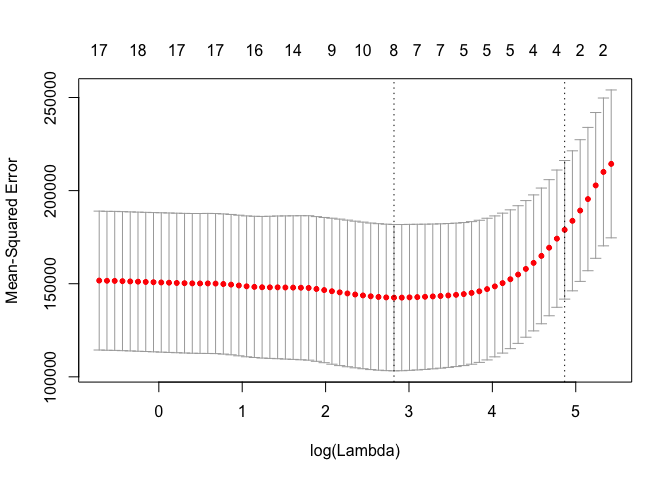
bestlam <- cv.out$lambda.min
lasso.pred <- predict(lasso.mod, s = bestlam, newx = x[test, ])
mean((lasso.pred - y.test)^2)
## [1] 100743.4
We can compare these results with ridge regression by examining the coefficient estimates.
out <- glmnet(x, y, alpha = 1, lambda = grid)
lasso.coef <- predict(out, type = "coefficients", s = bestlam)[1:20, ]
lasso.coef
##  (Intercept)        AtBat         Hits        HmRun         Runs
##   18.5394844    0.0000000    1.8735390    0.0000000    0.0000000
##          RBI        Walks        Years       CAtBat        CHits
##    0.0000000    2.2178444    0.0000000    0.0000000    0.0000000
##       CHmRun        CRuns         CRBI       CWalks      LeagueN
##    0.0000000    0.2071252    0.4130132    0.0000000    3.2666677
##    DivisionW      PutOuts      Assists       Errors   NewLeagueN
## -103.4845458    0.2204284    0.0000000    0.0000000    0.0000000
lasso.coef[lasso.coef != 0]
##  (Intercept)         Hits        Walks        CRuns         CRBI
##   18.5394844    1.8735390    2.2178444    0.2071252    0.4130132
##      LeagueN    DivisionW      PutOuts
##    3.2666677 -103.4845458    0.2204284
6.7 Lab 3: PCR and PLS Regression
The pls package provides functions for performing Principal Components Regression (PCR) and Partial Least Squares (PLS)
6.7.1 Principal Components Regression
We start by loading the pls package and calling pcr() on the Hitters dataset. The scale = TRUE parameter is used to standardize each predictor by dividing it by its sample standard deviation. The validation = "CV" parameter tells pcr() to perform cross-validation.
library(pls)
##
## Attaching package: 'pls'
##
## The following object is masked from 'package:stats':
##
##     loadings
set.seed(2)
pcr.fit <- pcr(Salary ~ ., data = Hitters, scale = TRUE, validation = "CV")
summary(pcr.fit)
## Data:    X dimension: 263 19
##  Y dimension: 263 1
## Fit method: svdpc
## Number of components considered: 19
##
## VALIDATION: RMSEP
## Cross-validated using 10 random segments.
##        (Intercept)  1 comps  2 comps  3 comps  4 comps  5 comps  6 comps
## CV             452    348.9    352.2    353.5    352.8    350.1    349.1
## adjCV          452    348.7    351.8    352.9    352.1    349.3    348.0
##        7 comps  8 comps  9 comps  10 comps  11 comps  12 comps  13 comps
## CV       349.6    350.9    352.9     353.8     355.0     356.2     363.5
## adjCV    348.5    349.8    351.6     352.3     353.4     354.5     361.6
##        14 comps  15 comps  16 comps  17 comps  18 comps  19 comps
## CV        355.2     357.4     347.6     350.1     349.2     352.6
## adjCV     352.8     355.2     345.5     347.6     346.7     349.8
##
## TRAINING: % variance explained
##         1 comps  2 comps  3 comps  4 comps  5 comps  6 comps  7 comps
## X         38.31    60.16    70.84    79.03    84.29    88.63    92.26
## Salary    40.63    41.58    42.17    43.22    44.90    46.48    46.69
##         8 comps  9 comps  10 comps  11 comps  12 comps  13 comps  14 comps
## X         94.96    96.28     97.26     97.98     98.65     99.15     99.47
## Salary    46.75    46.86     47.76     47.82     47.85     48.10     50.40
##         15 comps  16 comps  17 comps  18 comps  19 comps
## X          99.75     99.89     99.97     99.99    100.00
## Salary     50.55     53.01     53.85     54.61     54.61
We can plot the fitted model with validationplot().
validationplot(pcr.fit, val.type = "MSEP")
We can also perform PCR on a dataset split between training and test subsets. The syntax is identical to the previous exercise with the addition of a subset parameter indicating that the model should be estimated using only the training subset.
set.seed(1)
pcr.fit <- pcr(Salary ~ ., data = Hitters, subset = train, scale = TRUE, validation = "CV")
validationplot(pcr.fit, val.type = "MSEP")

We can calculate the MSE by predicting the y with a value for ncomp that results in the lowest cross-validation error.
pcr.pred <- predict(pcr.fit, x[test, ], ncomp = 7)
mean((pcr.pred - y.test)^2)
## [1] 96556.22
pcr.fit <- pcr(y ~ x, scale = TRUE, ncomp = 7)
summary(pcr.fit)
## Data:    X dimension: 263 19
##  Y dimension: 263 1
## Fit method: svdpc
## Number of components considered: 7
## TRAINING: % variance explained
##    1 comps  2 comps  3 comps  4 comps  5 comps  6 comps  7 comps
## X    38.31    60.16    70.84    79.03    84.29    88.63    92.26
## y    40.63    41.58    42.17    43.22    44.90    46.48    46.69
6.7.2 Partial Least Squares
Partial Least Squares is also provided by the pls package, and has the same syntax as the pcr() function. We fit a PLS model using the plsr() function.
set.seed(1)
pls.fit <- plsr(Salary ~ ., data = Hitters, subset = train, scale = TRUE, validation = "CV")
summary(pls.fit)
## Data:    X dimension: 131 19
##  Y dimension: 131 1
## Fit method: kernelpls
## Number of components considered: 19
##
## VALIDATION: RMSEP
## Cross-validated using 10 random segments.
##        (Intercept)  1 comps  2 comps  3 comps  4 comps  5 comps  6 comps
## CV           464.6    394.2    391.5    393.1    395.0    415.0    424.0
## adjCV        464.6    393.4    390.2    391.1    392.9    411.5    418.8
##        7 comps  8 comps  9 comps  10 comps  11 comps  12 comps  13 comps
## CV       424.5    415.8    404.6     407.1     412.0     414.4     410.3
## adjCV    418.9    411.4    400.7     402.2     407.2     409.3     405.6
##        14 comps  15 comps  16 comps  17 comps  18 comps  19 comps
## CV        406.2     408.6     410.5     408.8     407.8     410.2
## adjCV     401.8     403.9     405.6     404.1     403.2     405.5
##
## TRAINING: % variance explained
##         1 comps  2 comps  3 comps  4 comps  5 comps  6 comps  7 comps
## X         38.12    53.46    66.05    74.49    79.33    84.56    87.09
## Salary    33.58    38.96    41.57    42.43    44.04    45.59    47.05
##         8 comps  9 comps  10 comps  11 comps  12 comps  13 comps  14 comps
## X         90.74    92.55     93.94     97.23     97.88     98.35     98.85
## Salary    47.53    48.42     49.68     50.04     50.54     50.78     50.92
##         15 comps  16 comps  17 comps  18 comps  19 comps
## X          99.11     99.43     99.78     99.99    100.00
## Salary     51.04     51.11     51.15     51.16     51.18
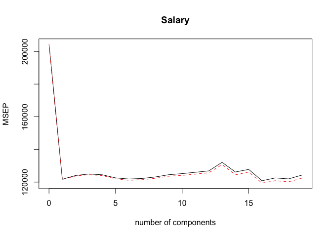
validationplot(pls.fit, val.type = "MSEP")

We perform cross-valiation on the test set in the same way and determine that the lowest cross-validation error is obtained with 2 components.
pls.pred <- predict(pls.fit, x[test, ], ncomp = 2)
mean((pls.pred - y.test)^2)
## [1] 101417.5
We can now run PLS on the full dataset with 2 components and display the summary of the results.
pls.fit <- plsr(Salary ~ ., data = Hitters, scale = TRUE, ncomp = 2)
summary(pls.fit)
## Data:    X dimension: 263 19
##  Y dimension: 263 1
## Fit method: kernelpls
## Number of components considered: 2
## TRAINING: % variance explained
##         1 comps  2 comps
## X         38.08    51.03
## Salary    43.05    46.40