An Introduction to Statistical Learning:

6.8 Exercises

Exercise 8

library("ISLR")
library("leaps")
library("glmnet")

## Loading required package: Matrix
## Loading required package: foreach
## Loaded glmnet 2.0-2

set.seed(0)

n <- 100
X <- rnorm(n)
epsilon <- 0.1 * rnorm(n)

beta_0 <- 1
beta_1 <- -0.1
beta_2 <- +0.05
beta_3 <- 0.75

Y <- beta_0 + beta_1 * X + beta_2 * X^2 + beta_3 * X^3 + epsilon

DF <- data.frame(Y = Y, X = X, X2 = X^2, X3 = X^3, X4 = X^4, X5 = X^5, X6 = X^6, X7 = X^7, X8 = X^8, X9 = X^9, X10 = X^10)

# Use the validation approach with regsubsets
train <- sample(c(TRUE, FALSE), n, rep = TRUE)  # will roughly assign TRUE to one-half of the data (FALSE to the other half).
test <- (!train)


# -- Apply best subset selection: --
regfit.full <- regsubsets(Y ~ ., data = DF[train, ], nvmax = 10)
print(summary(regfit.full))

## Subset selection object
## Call: regsubsets.formula(Y ~ ., data = DF[train, ], nvmax = 10)
## 10 Variables  (and intercept)
##     Forced in Forced out
## X       FALSE      FALSE
## X2      FALSE      FALSE
## X3      FALSE      FALSE
## X4      FALSE      FALSE
## X5      FALSE      FALSE
## X6      FALSE      FALSE
## X7      FALSE      FALSE
## X8      FALSE      FALSE
## X9      FALSE      FALSE
## X10     FALSE      FALSE
## 1 subsets of each size up to 10
## Selection Algorithm: exhaustive
##           X   X2  X3  X4  X5  X6  X7  X8  X9  X10
## 1  ( 1 )  " " " " "*" " " " " " " " " " " " " " "
## 2  ( 1 )  "*" " " "*" " " " " " " " " " " " " " "
## 3  ( 1 )  "*" "*" "*" " " " " " " " " " " " " " "
## 4  ( 1 )  " " "*" "*" " " "*" " " "*" " " " " " "
## 5  ( 1 )  " " "*" "*" "*" "*" " " " " " " "*" " "
## 6  ( 1 )  " " "*" "*" " " "*" "*" " " "*" "*" " "
## 7  ( 1 )  "*" "*" "*" " " "*" "*" " " "*" "*" " "
## 8  ( 1 )  " " "*" "*" " " "*" "*" "*" "*" "*" "*"
## 9  ( 1 )  "*" "*" "*" " " "*" "*" "*" "*" "*" "*"
## 10  ( 1 ) "*" "*" "*" "*" "*" "*" "*" "*" "*" "*"

reg.summary <- summary(regfit.full)

# Test models on the validation set:
test.mat <- model.matrix(Y ~ ., data = DF[test, ])
val.errors <- rep(NA, 10)
for (ii in 1:10) {
    coefi <- coef(regfit.full, id = ii)
    pred <- test.mat[, names(coefi)] %*% coefi
    val.errors[ii] <- mean((DF$Y[test] - pred)^2)
}
print("best subset validation errors")

## [1] "best subset validation errors"

print(val.errors)

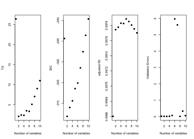
##  [1] 0.015567409 0.013245221 0.009026844 0.017169840 0.065102301
##  [6] 5.962097578 5.599171828 0.010197576 0.328677632 0.055217617

k <- which.min(val.errors)
print(k)

## [1] 3

print(coef(regfit.full, id = k))

## (Intercept)           X          X2          X3 
##  1.01506706 -0.11855671  0.02753875  0.76721123

old.par <- par(mfrow = c(1, 4))
# plot( reg.summary$rss, xlab='Number of variables', ylab='RSS' )
plot(reg.summary$cp, xlab = "Number of variables", ylab = "Cp", pch = 19)
plot(reg.summary$bic, xlab = "Number of variables", ylab = "BIC", pch = 19)
plot(reg.summary$adjr2, xlab = "Number of variables", ylab = "adjusted R2", pch = 19)

plot(val.errors, xlab = "Number of variables", ylab = "Validation Errors", pch = 19)

par(mfrow = c(1, 1))

# -- Now apply foward selection on the training set: --
regfit.forward <- regsubsets(Y ~ ., data = DF[train, ], nvmax = 10, method = "forward")
print(summary(regfit.forward))

## Subset selection object
## Call: regsubsets.formula(Y ~ ., data = DF[train, ], nvmax = 10, method = "forward")
## 10 Variables  (and intercept)
##     Forced in Forced out
## X       FALSE      FALSE
## X2      FALSE      FALSE
## X3      FALSE      FALSE
## X4      FALSE      FALSE
## X5      FALSE      FALSE
## X6      FALSE      FALSE
## X7      FALSE      FALSE
## X8      FALSE      FALSE
## X9      FALSE      FALSE
## X10     FALSE      FALSE
## 1 subsets of each size up to 10
## Selection Algorithm: forward
##           X   X2  X3  X4  X5  X6  X7  X8  X9  X10
## 1  ( 1 )  " " " " "*" " " " " " " " " " " " " " "
## 2  ( 1 )  "*" " " "*" " " " " " " " " " " " " " "
## 3  ( 1 )  "*" "*" "*" " " " " " " " " " " " " " "
## 4  ( 1 )  "*" "*" "*" "*" " " " " " " " " " " " "
## 5  ( 1 )  "*" "*" "*" "*" "*" " " " " " " " " " "
## 6  ( 1 )  "*" "*" "*" "*" "*" " " " " " " "*" " "
## 7  ( 1 )  "*" "*" "*" "*" "*" " " " " "*" "*" " "
## 8  ( 1 )  "*" "*" "*" "*" "*" "*" " " "*" "*" " "
## 9  ( 1 )  "*" "*" "*" "*" "*" "*" "*" "*" "*" " "
## 10  ( 1 ) "*" "*" "*" "*" "*" "*" "*" "*" "*" "*"

reg.summary <- summary(regfit.forward)

# Test models on the validation set:
test.mat <- model.matrix(Y ~ ., data = DF[test, ])
val.errors <- rep(NA, 10)
for (ii in 1:10) {
    coefi <- coef(regfit.forward, id = ii)
    pred <- test.mat[, names(coefi)] %*% coefi
    val.errors[ii] <- mean((DF$Y[test] - pred)^2)
}
print("forward selection validation errors")

## [1] "forward selection validation errors"

print(val.errors)

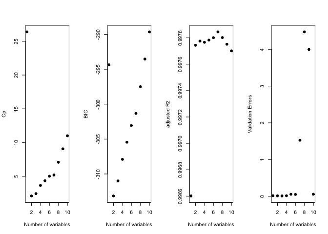
##  [1] 0.015567409 0.013245221 0.009026844 0.014540813 0.055005227
##  [6] 0.049894349 1.525498490 4.476027607 3.997884857 0.055217617

k <- which.min(val.errors)
print(k)

## [1] 3

print(coef(regfit.forward, id = k))

## (Intercept)           X          X2          X3 
##  1.01506706 -0.11855671  0.02753875  0.76721123

old.par <- par(mfrow = c(1, 4))
# plot( reg.summary$rss, xlab='Number of variables', ylab='RSS' )
plot(reg.summary$cp, xlab = "Number of variables", ylab = "Cp", pch = 19)
plot(reg.summary$bic, xlab = "Number of variables", ylab = "BIC", pch = 19)
plot(reg.summary$adjr2, xlab = "Number of variables", ylab = "adjusted R2", pch = 19)

plot(val.errors, xlab = "Number of variables", ylab = "Validation Errors", pch = 19)

par(mfrow = c(1, 1))


# -- Now apply backwards selection to the training set: --
regfit.backward <- regsubsets(Y ~ ., data = DF[train, ], nvmax = 10, method = "backward")
print(summary(regfit.backward))

## Subset selection object
## Call: regsubsets.formula(Y ~ ., data = DF[train, ], nvmax = 10, method = "backward")
## 10 Variables  (and intercept)
##     Forced in Forced out
## X       FALSE      FALSE
## X2      FALSE      FALSE
## X3      FALSE      FALSE
## X4      FALSE      FALSE
## X5      FALSE      FALSE
## X6      FALSE      FALSE
## X7      FALSE      FALSE
## X8      FALSE      FALSE
## X9      FALSE      FALSE
## X10     FALSE      FALSE
## 1 subsets of each size up to 10
## Selection Algorithm: backward
##           X   X2  X3  X4  X5  X6  X7  X8  X9  X10
## 1  ( 1 )  " " " " "*" " " " " " " " " " " " " " "
## 2  ( 1 )  " " " " "*" " " "*" " " " " " " " " " "
## 3  ( 1 )  "*" "*" "*" " " " " " " " " " " " " " "
## 4  ( 1 )  " " "*" "*" " " "*" " " "*" " " " " " "
## 5  ( 1 )  " " "*" "*" " " "*" "*" "*" " " " " " "
## 6  ( 1 )  " " "*" "*" " " "*" "*" "*" "*" " " " "
## 7  ( 1 )  " " "*" "*" " " "*" "*" "*" "*" " " "*"
## 8  ( 1 )  " " "*" "*" " " "*" "*" "*" "*" "*" "*"
## 9  ( 1 )  "*" "*" "*" " " "*" "*" "*" "*" "*" "*"
## 10  ( 1 ) "*" "*" "*" "*" "*" "*" "*" "*" "*" "*"

reg.summary <- summary(regfit.backward)

# Test models on the validation set:
test.mat <- model.matrix(Y ~ ., data = DF[test, ])
val.errors <- rep(NA, 10)
for (ii in 1:10) {
    coefi <- coef(regfit.backward, id = ii)
    pred <- test.mat[, names(coefi)] %*% coefi
    val.errors[ii] <- mean((DF$Y[test] - pred)^2)
}
print("backwards selection validation errors")

## [1] "backwards selection validation errors"

print(val.errors)

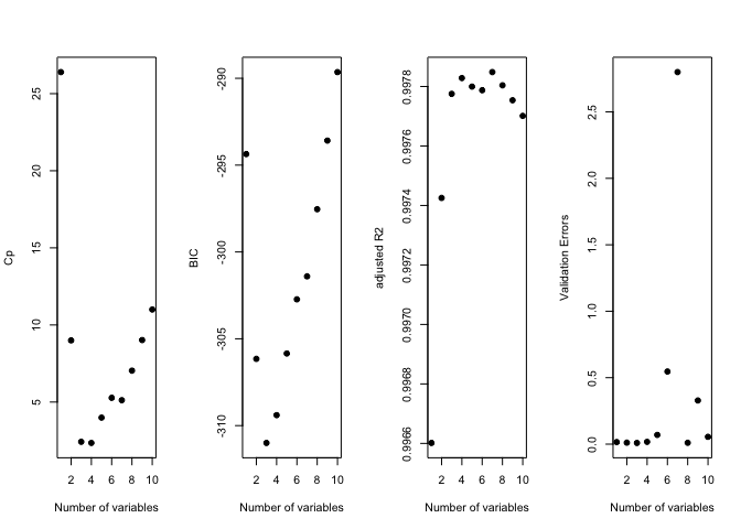
##  [1] 0.015567409 0.011250512 0.009026844 0.017169840 0.069259376
##  [6] 0.546418670 2.799471622 0.010197576 0.328677632 0.055217617

k <- which.min(val.errors)
print(k)

## [1] 3

print(coef(regfit.backward, id = k))

## (Intercept)           X          X2          X3 
##  1.01506706 -0.11855671  0.02753875  0.76721123

old.par <- par(mfrow = c(1, 4))
# plot( reg.summary$rss, xlab='Number of variables', ylab='RSS' )
plot(reg.summary$cp, xlab = "Number of variables", ylab = "Cp", pch = 19)
plot(reg.summary$bic, xlab = "Number of variables", ylab = "BIC", pch = 19)
plot(reg.summary$adjr2, xlab = "Number of variables", ylab = "adjusted R2", pch = 19)

plot(val.errors, xlab = "Number of variables", ylab = "Validation Errors", pch = 19)

par(mfrow = c(1, 1))


# -- Now apply the lasso to our training set: --

# First fit the lasso model for all of the given lambda values :
grid <- 10^seq(10, -2, length = 100)  # a grid of lambda values 
Y <- DF$Y
MM <- model.matrix(Y ~ ., data = DF)  # the predictors as a datamatrix 
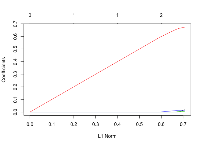
lasso.mod <- glmnet(MM, Y, alpha = 1, lambda = grid)
plot(lasso.mod)  # plots the extracted coefficients as a function of lambda

# Apply cross validation (to pick the best value of lambda):
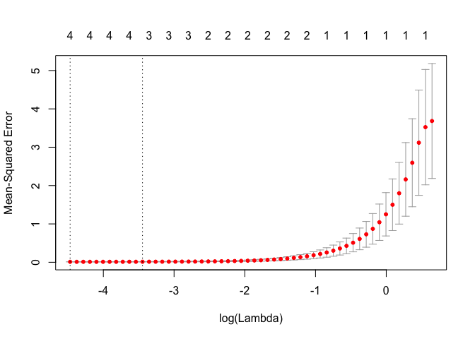
cv.out <- cv.glmnet(MM, Y, alpha = 1)
bestlam <- cv.out$lambda.1se
print("lasso CV best value of lambda (one standard error)")

## [1] "lasso CV best value of lambda (one standard error)"

print(bestlam)

## [1] 0.03186245

plot(cv.out)

# Extract the optimal coefficients used:
lasso.coef <- predict(lasso.mod, type = "coefficients", s = bestlam)
print(lasso.coef)

## 12 x 1 sparse Matrix of class "dgCMatrix"
##                       1
## (Intercept) 1.026020037
## (Intercept) .          
## X           .          
## X2          0.004179690
## X3          0.664868098
## X4          0.003606719
## X5          0.011344145
## X6          .          
## X7          .          
## X8          .          
## X9          .          
## X10         .

# Part (f) Try a different regression function:
X <- rnorm(n)
epsilon <- 0.1 * rnorm(n)

beta_0 <- 1
beta_7 <- 2.5
Y <- beta_0 + beta_7 * X^7 + epsilon
DF <- data.frame(Y = Y, X = X, X2 = X^2, X3 = X^3, X4 = X^4, X5 = X^5, X6 = X^6, X7 = X^7, X8 = X^8, X9 = X^9, X10 = X^10)

train <- sample(c(TRUE, FALSE), n, rep = TRUE)  # will roughly assign TRUE to one-half of the data (FALSE to the other half).
test <- (!train)

# Best subset selection:
regfit.full <- regsubsets(Y ~ ., data = DF[train, ], nvmax = 10)
print(summary(regfit.full))

## Subset selection object
## Call: regsubsets.formula(Y ~ ., data = DF[train, ], nvmax = 10)
## 10 Variables  (and intercept)
##     Forced in Forced out
## X       FALSE      FALSE
## X2      FALSE      FALSE
## X3      FALSE      FALSE
## X4      FALSE      FALSE
## X5      FALSE      FALSE
## X6      FALSE      FALSE
## X7      FALSE      FALSE
## X8      FALSE      FALSE
## X9      FALSE      FALSE
## X10     FALSE      FALSE
## 1 subsets of each size up to 10
## Selection Algorithm: exhaustive
##           X   X2  X3  X4  X5  X6  X7  X8  X9  X10
## 1  ( 1 )  " " " " " " " " " " " " "*" " " " " " "
## 2  ( 1 )  "*" " " " " " " " " " " "*" " " " " " "
## 3  ( 1 )  "*" " " " " " " "*" " " "*" " " " " " "
## 4  ( 1 )  " " " " "*" " " "*" " " "*" " " "*" " "
## 5  ( 1 )  " " " " "*" "*" "*" " " "*" " " "*" " "
## 6  ( 1 )  " " " " " " " " "*" "*" "*" "*" "*" "*"
## 7  ( 1 )  " " "*" " " "*" "*" "*" "*" " " "*" "*"
## 8  ( 1 )  "*" "*" " " "*" "*" "*" "*" " " "*" "*"
## 9  ( 1 )  "*" "*" "*" "*" "*" "*" "*" " " "*" "*"
## 10  ( 1 ) "*" "*" "*" "*" "*" "*" "*" "*" "*" "*"

# Test best subset models on the validation set:
test.mat <- model.matrix(Y ~ ., data = DF[test, ])
val.errors <- rep(NA, 10)
for (ii in 1:10) {
    coefi <- coef(regfit.full, id = ii)
    pred <- test.mat[, names(coefi)] %*% coefi
    val.errors[ii] <- mean((DF$Y[test] - pred)^2)
}
print("best subsets validation errors")

## [1] "best subsets validation errors"

print(val.errors)

##  [1] 0.01151953 0.01334971 0.01514501 0.06420174 0.09905791 1.86716273
##  [7] 0.62617621 0.58059869 0.53819549 1.05507636

k <- which.min(val.errors)
print(k)

## [1] 1

print("best subsets optimal coefficients")

## [1] "best subsets optimal coefficients"

print(coef(regfit.full, id = k))  # print the coefficients of the best model

## (Intercept)          X7 
##   0.9840339   2.5000261

print(val.errors[k])

## [1] 0.01151953

# Using the lasso technique:

# First apply cross validation (to find the optimal value of lambda):
MM <- model.matrix(Y ~ ., data = DF)

cv.out <- cv.glmnet(MM, Y, alpha = 1)
plot(cv.out)

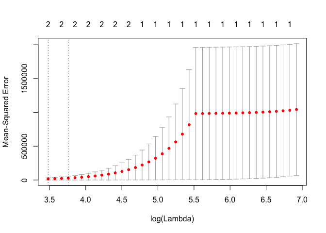
bestlam <- cv.out$lambda.1se
print("best lambda (1 se)")

## [1] "best lambda (1 se)"

print(bestlam)

## [1] 42.84324

# Now fit the lasso with this value of lambda:
lasso.mod <- glmnet(MM, Y, alpha = 1)

lasso.coef <- predict(lasso.mod, type = "coefficients", s = bestlam)
print("lasso optimal coefficients")

## [1] "lasso optimal coefficients"

print(lasso.coef)

## 12 x 1 sparse Matrix of class "dgCMatrix"
##                     1
## (Intercept) 5.3888292
## (Intercept) .        
## X           .        
## X2          .        
## X3          .        
## X4          .        
## X5          .        
## X6          0.2125842
## X7          2.3286883
## X8          .        
## X9          .        
## X10         .

print("I do not think the predict method is working correctly...")

## [1] "I do not think the predict method is working correctly..."

lasso.predict <- predict(lasso.mod, s = bestlam, newx = MM)
print("lasso RSS error")

## [1] "lasso RSS error"

print(mean((Y - lasso.predict)^2))

## [1] 1839.887

Exercise 9

library(pls)

## 
## Attaching package: 'pls'
## 
## The following object is masked from 'package:stats':
## 
##     loadings

set.seed(0)

n <- dim(College)[1]
p <- dim(College)[2]

train <- sample(c(TRUE, FALSE), n, rep = TRUE)  # will roughly assign TRUE to one-half of the data (FALSE to the other half).
test <- (!train)

College_train <- College[train, ]
College_test <- College[test, ]

# Part (b):
m <- lm(Apps ~ ., data = College_train)

Y_hat <- predict(m, newdata = College_test)
MSE <- mean((College_test$Apps - Y_hat)^2)
print(sprintf("Linear model test MSE= %10.3f", MSE))

## [1] "Linear model test MSE= 1615966.966"

# Part (c):
Y <- College_train$Apps
MM <- model.matrix(Apps ~ ., data = College_train)
cv.out <- cv.glmnet(MM, Y, alpha = 0)
plot(cv.out)

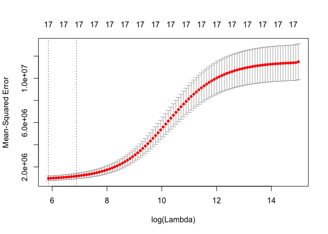
bestlam <- cv.out$lambda.1se
# print( 'ridge regression CV best value of lambda (one standard error)' ) print( bestlam )

ridge.mod <- glmnet(MM, Y, alpha = 0)

Y_hat <- predict(ridge.mod, s = bestlam, newx = model.matrix(Apps ~ ., data = College_test))
MSE <- mean((College_test$Apps - Y_hat)^2)
print(sprintf("Ridge regression test MSE= %10.3f", MSE))

## [1] "Ridge regression test MSE= 3318015.663"

# Part (d):
cv.out <- cv.glmnet(MM, Y, alpha = 1)
plot(cv.out)

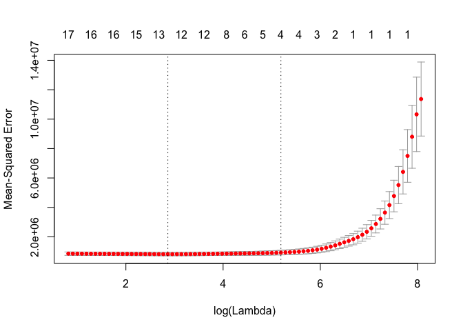
bestlam <- cv.out$lambda.1se
# print( 'lasso CV best value of lambda (one standard error)' ) print( bestlam )

lasso.mod <- glmnet(MM, Y, alpha = 1)

Y_hat <- predict(lasso.mod, s = bestlam, newx = model.matrix(Apps ~ ., data = College_test))
MSE <- mean((College_test$Apps - Y_hat)^2)
print(sprintf("Lasso regression test MSE= %10.3f", MSE))

## [1] "Lasso regression test MSE= 2018489.732"

print("lasso coefficients")

## [1] "lasso coefficients"

print(predict(lasso.mod, type = "coefficients", s = bestlam))

## 19 x 1 sparse Matrix of class "dgCMatrix"
##                         1
## (Intercept) -515.67319420
## (Intercept)    .         
## PrivateYes     .         
## Accept         1.26431392
## Enroll         .         
## Top10perc     14.89903622
## Top25perc      .         
## F.Undergrad    0.01925533
## P.Undergrad    .         
## Outstate       .         
## Room.Board     .         
## Books          .         
## Personal       .         
## PhD            .         
## Terminal       .         
## S.F.Ratio      .         
## perc.alumni    .         
## Expend         0.04586867
## Grad.Rate      .

# Part (e):
pcr.mod <- pcr(Apps ~ ., data = College_train, scale = TRUE, validation = "CV")

# Use this to select the number of components to include ... looks like CV suggests we should use ALL predictors
validationplot(pcr.mod, val.type = "MSEP")

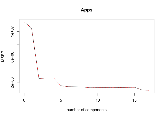
ncomp <- 17
Y_hat <- predict(pcr.mod, College_test, ncomp = ncomp)
MSE <- mean((College_test$Apps - Y_hat)^2)
print(sprintf("PCR (with ncomp= %5d) test MSE= %10.3f", ncomp, MSE))

## [1] "PCR (with ncomp=    17) test MSE= 1615966.966"

# Part (f):
pls.mod <- plsr(Apps ~ ., data = College_train, scale = TRUE, validation = "CV")

# Use this to select the number of components to include ... looks like CV suggests the best is to use ALL predictors but there is
# not much change in moving from ~ 5 predictors to 17 so we will take 10 (somewhere in the middle)
validationplot(pls.mod, val.type = "MSEP")

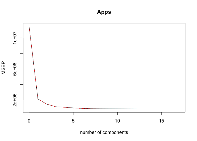
ncomp <- 10
Y_hat <- predict(pls.mod, College_test, ncomp = ncomp)
MSE <- mean((College_test$Apps - Y_hat)^2)
print(sprintf("PLS (with ncomp= %5d) test MSE= %10.3f", ncomp, MSE))

## [1] "PLS (with ncomp=    10) test MSE= 1601425.747"

Exercise 10

set.seed(0)

# The sample size and the number of features:
n <- 1000
p <- 20

# Create the true value of beta (and zero out half of the entries):
beta_truth <- rnorm(p + 1)  # add one for the constant beta_0 
zero_locations <- c(2, 3, 4, 7, 8, 11, 12, 15, 17, 20)
beta_truth[zero_locations] <- 0
# For debugging lets check that we can recover our coefficients: beta_truth = rep(0,p+1); beta_truth[1] = 1.5; beta_truth[10] = 3.5;
# beta_truth[15] = -3.4
print("True values for beta (beta_0-beta_20):")

## [1] "True values for beta (beta_0-beta_20):"

print(beta_truth)

##  [1]  1.262954285  0.000000000  0.000000000  0.000000000  0.414641434
##  [6] -1.539950042  0.000000000  0.000000000 -0.005767173  2.404653389
## [11]  0.000000000  0.000000000 -1.147657009 -0.289461574  0.000000000
## [16] -0.411510833  0.000000000 -0.891921127  0.435683299  0.000000000
## [21] -0.224267885

# Generate some input features and an output response:
X <- c(rep(1, n), rnorm(n * p))  # make leading column of ones 
X <- matrix(X, nrow = n, ncol = (p + 1), byrow = FALSE)

Y <- X %*% beta_truth + rnorm(n)

# Create a dataframe with this data:
DF <- data.frame(Y, X[, -1])  # drop the column of ones 

train_inds <- sample(1:n, 100)
test_inds <- (1:n)[-train_inds]

# -- Apply best subset selection using the training data: --
regfit.full <- regsubsets(Y ~ ., data = DF[train_inds, ], nvmax = 20)
# print( summary( regfit.full ) )
reg.summary <- summary(regfit.full)

# Plot the in-sample MSE:
training.mat <- model.matrix(Y ~ ., data = DF[train_inds, ])
training.errors <- rep(NA, 20)
for (ii in 1:20) {
    coefi <- coef(regfit.full, id = ii)
    pred <- training.mat[, names(coefi)] %*% coefi
    training.errors[ii] <- mean((DF$Y[train_inds] - pred)^2)
}
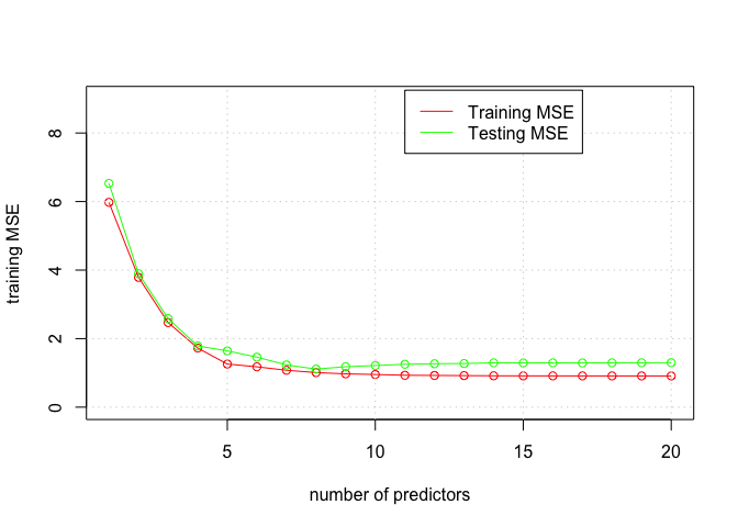
print("best subset training MSE")

## [1] "best subset training MSE"

print(training.errors)

##  [1] 5.9770059 3.7871159 2.4678405 1.7251665 1.2576488 1.1772519 1.0768021
##  [8] 1.0087222 0.9721521 0.9530143 0.9304660 0.9254522 0.9206935 0.9152359
## [15] 0.9133050 0.9125718 0.9117938 0.9112271 0.9108313 0.9106024

plot(1:20, training.errors, xlab = "number of predictors", ylab = "training MSE", type = "o", col = "red", ylim = c(0, 9))

# Test models on the validation set:
test.mat <- model.matrix(Y ~ ., data = DF[test_inds, ])
val.errors <- rep(NA, 20)
for (ii in 1:20) {
    coefi <- coef(regfit.full, id = ii)
    pred <- test.mat[, names(coefi)] %*% coefi
    val.errors[ii] <- mean((DF$Y[test_inds] - pred)^2)
}
print("best subset validation MSE")

## [1] "best subset validation MSE"

print(val.errors)

##  [1] 6.531306 3.895918 2.584956 1.787702 1.642511 1.458888 1.232284
##  [8] 1.111670 1.180321 1.214303 1.251878 1.267629 1.274193 1.293091
## [15] 1.290385 1.292731 1.290206 1.294843 1.295492 1.297954

k <- which.min(val.errors)
print(k)

## [1] 8

print(coef(regfit.full, id = k))

## (Intercept)          X4          X5          X9         X12         X13 
##   1.3210455   0.4132288  -1.5880109   2.4639393  -1.1455077  -0.2815162 
##         X15         X17         X18 
##  -0.3589236  -1.0286318   0.6142240

points(1:20, val.errors, xlab = "number of predictors", ylab = "testing MSE", type = "o", col = "green")

grid()
legend(11, 9.25, c("Training MSE", "Testing MSE"), col = c("red", "green"), lty = c(1, 1))

# Part (g):
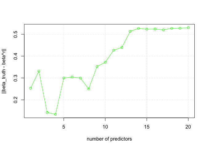
nms <- colnames(DF)
nms[1] <- "(Intercept)"
names(beta_truth) <- nms

norm.beta.diff <- rep(NA, 20)
for (ii in 1:20) {
    coefi <- coef(regfit.full, id = ii)
    norm.beta.diff[ii] <- sqrt(sum((beta_truth[names(coefi)] - coefi)^2))
}

plot(1:20, norm.beta.diff, xlab = "number of predictors", ylab = "||beta_truth - beta^r||", type = "o", col = "green")
grid()

Exercise 11

library(MASS)

set.seed(0)

n <- dim(Boston)[1]
p <- dim(Boston)[2]

train <- sample(c(TRUE, FALSE), n, rep = TRUE)  # will roughly assign TRUE to one-half of the data (FALSE to the other half).
test <- (!train)

Boston_train <- Boston[train, ]
Boston_test <- Boston[test, ]

# The full linear model:
m <- lm(crim ~ ., data = Boston_train)

Y_hat <- predict(m, newdata = Boston_test)
MSE <- mean((Boston_test$crim - Y_hat)^2)
print(sprintf("Linear model test MSE= %10.3f", MSE))

## [1] "Linear model test MSE=     34.996"

# Ridge regression:
Y <- Boston_train$crim
MM <- model.matrix(crim ~ ., data = Boston_train)
cv.out <- cv.glmnet(MM, Y, alpha = 0)
plot(cv.out)

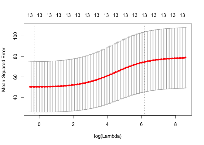
bestlam <- cv.out$lambda.1se
# print( 'ridge regression CV best value of lambda (one standard error)' ) print( bestlam )

ridge.mod <- glmnet(MM, Y, alpha = 0)

Y_hat <- predict(ridge.mod, s = bestlam, newx = model.matrix(crim ~ ., data = Boston_test))
MSE <- mean((Boston_test$crim - Y_hat)^2)
print(sprintf("Ridge regression test MSE= %10.3f", MSE))

## [1] "Ridge regression test MSE=     63.826"

# The Lasso:
cv.out <- cv.glmnet(MM, Y, alpha = 1)
plot(cv.out)

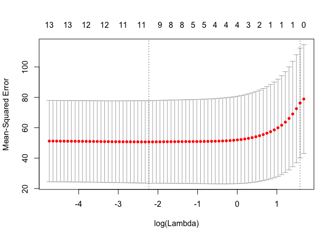
bestlam <- cv.out$lambda.1se
# print( 'lasso CV best value of lambda (one standard error)' ) print( bestlam )

lasso.mod <- glmnet(MM, Y, alpha = 1)

Y_hat <- predict(lasso.mod, s = bestlam, newx = model.matrix(crim ~ ., data = Boston_test))
MSE <- mean((Boston_test$crim - Y_hat)^2)
print(sprintf("Lasso regression test MSE= %10.3f", MSE))

## [1] "Lasso regression test MSE=     63.572"

print("lasso coefficients")

## [1] "lasso coefficients"

print(predict(lasso.mod, type = "coefficients", s = bestlam))

## 15 x 1 sparse Matrix of class "dgCMatrix"
##                      1
## (Intercept) 3.07011734
## (Intercept) .         
## zn          .         
## indus       .         
## chas        .         
## nox         .         
## rm          .         
## age         .         
## dis         .         
## rad         0.05507813
## tax         .         
## ptratio     .         
## black       .         
## lstat       .         
## medv        .

# Principle Component Regression:
pcr.mod <- pcr(crim ~ ., data = Boston_train, scale = TRUE, validation = "CV")

# Use this to select the number of components to include ... looks like CV suggests we should use 3 predictors
validationplot(pcr.mod, val.type = "MSEP")

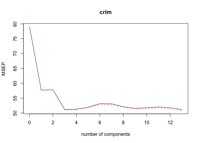
ncomp <- 3
Y_hat <- predict(pcr.mod, Boston_test, ncomp = ncomp)
MSE <- mean((Boston_test$crim - Y_hat)^2)
print(sprintf("PCR (with ncomp= %5d) test MSE= %10.3f", ncomp, MSE))

## [1] "PCR (with ncomp=     3) test MSE=     40.049"

# Paritial Least Squares:
pls.mod <- plsr(crim ~ ., data = Boston_train, scale = TRUE, validation = "CV")

# Use this to select the number of components to include ... looks like CV suggests the best is to use 5 predictors
validationplot(pls.mod, val.type = "MSEP")

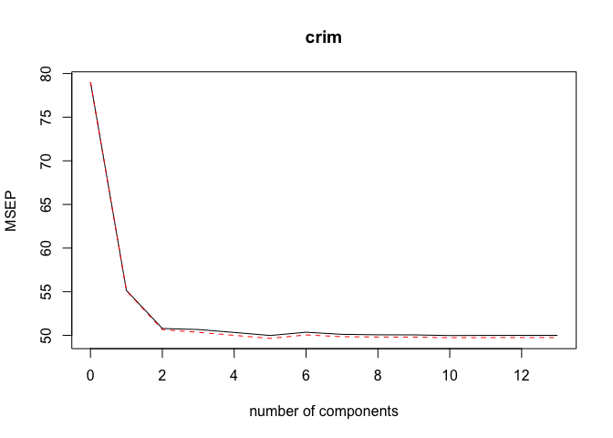
ncomp <- 5
Y_hat <- predict(pls.mod, Boston_test, ncomp = ncomp)
MSE <- mean((Boston_test$crim - Y_hat)^2)
print(sprintf("PLS (with ncomp= %5d) test MSE= %10.3f", ncomp, MSE))

## [1] "PLS (with ncomp=     5) test MSE=     35.258"