An Introduction to Statistical Learning:

5.4 Exercises

library(ISLR)

Exercise 5

library(boot)

set.seed(0)
Default <- na.omit(Default)

m0 <- glm(default ~ income + balance, data = Default, family = "binomial")
summary(m0)

## 
## Call:
## glm(formula = default ~ income + balance, family = "binomial", 
##     data = Default)
## 
## Deviance Residuals: 
##     Min       1Q   Median       3Q      Max  
## -2.4725  -0.1444  -0.0574  -0.0211   3.7245  
## 
## Coefficients:
##               Estimate Std. Error z value Pr(>|z|)    
## (Intercept) -1.154e+01  4.348e-01 -26.545  < 2e-16 ***
## income       2.081e-05  4.985e-06   4.174 2.99e-05 ***
## balance      5.647e-03  2.274e-04  24.836  < 2e-16 ***
## ---
## Signif. codes:  0 '***' 0.001 '**' 0.01 '*' 0.05 '.' 0.1 ' ' 1
## 
## (Dispersion parameter for binomial family taken to be 1)
## 
##     Null deviance: 2920.6  on 9999  degrees of freedom
## Residual deviance: 1579.0  on 9997  degrees of freedom
## AIC: 1585
## 
## Number of Fisher Scoring iterations: 8

validation_error_5b <- function() {
    # Predictors are income and balance

    # (i):
    n <- dim(Default)[1]
    training_samples <- sample(1:n, floor(n/2))
    validation_samples <- (1:n)[-training_samples]

    # (ii):
    m <- glm(default ~ income + balance, data = Default, family = "binomial", subset = training_samples)

    # Results from 'predict' are in terms of log odds or the logit tranformation of the probabilities
    predictions <- predict(m, newdata = Default[validation_samples, ])

    default <- factor(rep("No", length(validation_samples)), c("No", "Yes"))
    default[predictions > 0] <- factor("Yes", c("No", "Yes"))

    validation_error_rate <- mean(default != Default[validation_samples, ]$default)
}

v_error = validation_error_5b()

v_errors <- rep(0, 3)
for (i in 1:length(v_errors)) {
  v_errors[i] = validation_error_5b()
}

Validation set error is: 0.0268.

Three more estimates of the validation set error would give: 0.0236, 0.026, 0.0304.

validation_error_5d <- function() {
    # Predictors are income, balance, AND student

    # (i):
    n <- dim(Default)[1]
    training_samples <- sample(1:n, floor(n/2))
    validation_samples <- (1:n)[-training_samples]

    # (ii):
    m <- glm(default ~ income + balance + student, data = Default, family = "binomial", subset = training_samples)

    # Results from 'predict' are in terms of log odds or the logit tranformation of the probabilities
    predictions <- predict(m, newdata = Default[validation_samples, ])

    default <- factor(rep("No", length(validation_samples)), c("No", "Yes"))
    default[predictions > 0] <- factor("Yes", c("No", "Yes"))

    validation_error_rate <- mean(default != Default[validation_samples, ]$default)
}

v_error = validation_error_5d()

Using the predictor student, our validation set error is: 0.0272.

Exercise 6

set.seed(0)

Default <- na.omit(Default)

# Estimate the base model (to get standard errors of the coefficients):
m0 <- glm(default ~ income + balance, data = Default, family = "binomial")
summary(m0)

## 
## Call:
## glm(formula = default ~ income + balance, family = "binomial", 
##     data = Default)
## 
## Deviance Residuals: 
##     Min       1Q   Median       3Q      Max  
## -2.4725  -0.1444  -0.0574  -0.0211   3.7245  
## 
## Coefficients:
##               Estimate Std. Error z value Pr(>|z|)    
## (Intercept) -1.154e+01  4.348e-01 -26.545  < 2e-16 ***
## income       2.081e-05  4.985e-06   4.174 2.99e-05 ***
## balance      5.647e-03  2.274e-04  24.836  < 2e-16 ***
## ---
## Signif. codes:  0 '***' 0.001 '**' 0.01 '*' 0.05 '.' 0.1 ' ' 1
## 
## (Dispersion parameter for binomial family taken to be 1)
## 
##     Null deviance: 2920.6  on 9999  degrees of freedom
## Residual deviance: 1579.0  on 9997  degrees of freedom
## AIC: 1585
## 
## Number of Fisher Scoring iterations: 8

boot.fn <- function(data, index) {
    m <- glm(default ~ income + balance, data = data[index, ], family = "binomial")
    return(coefficients(m))
}
boot.fn(Default, 1:10000)  # test our boot function

##   (Intercept)        income       balance 
## -1.154047e+01  2.080898e-05  5.647103e-03

boot(Default, boot.fn, 1000)

## 
## ORDINARY NONPARAMETRIC BOOTSTRAP
## 
## 
## Call:
## boot(data = Default, statistic = boot.fn, R = 1000)
## 
## 
## Bootstrap Statistics :
##          original        bias     std. error
## t1* -1.154047e+01 -3.566749e-02 4.408921e-01
## t2*  2.080898e-05  2.589821e-07 4.968550e-06
## t3*  5.647103e-03  1.518670e-05 2.332941e-04

Exercise 7

set.seed(0)

# Part (a):
m_0 <- glm(Direction ~ Lag1 + Lag2, data = Weekly, family = "binomial")

# Part (b):
m_loocv <- glm(Direction ~ Lag1 + Lag2, data = Weekly[-1, ], family = "binomial")

weekly_predict = predict(m_loocv, newdata = Weekly[1, ]) > 0
weekly_direction = Weekly[1, ]$Direction

Prediction on first sample is TRUE (1=>Up; 0=>Down)

First samples true direction is Down

n <- dim(Weekly)[1]
number_of_errors <- 0
for (ii in 1:n) {
    m_loocv <- glm(Direction ~ Lag1 + Lag2, data = Weekly[-ii, ], family = "binomial")

    error_1 <- (predict(m_loocv, newdata = Weekly[ii, ]) > 0) & (Weekly[ii, ]$Direction == "Down")
    error_2 <- (predict(m_loocv, newdata = Weekly[ii, ]) < 0) & (Weekly[ii, ]$Direction == "Up")
    if (error_1 | error_2) {
        number_of_errors <- number_of_errors + 1
    }
}
LOOCV_test_error_rate = sprintf("%10.6f", number_of_errors/n)

LOOCV test error rate = 0.449954

Exercise 8

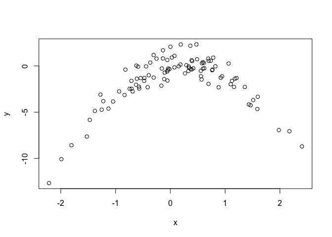
# Part (a):
set.seed(1)

x <- rnorm(100)
y <- x - 2 * x^2 + rnorm(100)

plot(x, y)

# dev.off()

DF <- data.frame(y = y, x = x)

# Do cross-validation on each model:
m_i <- glm(y ~ x, data = DF)
cv.err <- cv.glm(DF, m_i)
result = sprintf("%10.6f", cv.err$delta[1])

Model (i): cv output= 7.288162

m_ii <- glm(y ~ x + I(x^2), data = DF)
cv.err <- cv.glm(DF, m_ii)
result = sprintf("%10.6f", cv.err$delta[1])

Model (ii): cv output= 0.937424

m_iii <- glm(y ~ x + I(x^2) + I(x^3), data = DF)
cv.err <- cv.glm(DF, m_iii)
result = sprintf("%10.6f", cv.err$delta[1])

Model (iii): cv output= 0.956622

m_iv <- glm(y ~ x + I(x^2) + I(x^3) + I(x^4), data = DF)
cv.err <- cv.glm(DF, m_iv)
result = sprintf("%10.6f", cv.err$delta[1])

Model (iv): cv output= 0.953905

Exercise 9

library(MASS)

Boston <- na.omit(Boston)

# Part (a):
mu_hat <- mean(Boston$medv)

# Part (b):
n <- dim(Boston)[1]
mu_se <- sd(Boston$medv)/sqrt(n)

mean_boot.fn <- function(data, index) {
    mean(data[index])
}

boot(Boston$medv, mean_boot.fn, 1000)

## 
## ORDINARY NONPARAMETRIC BOOTSTRAP
## 
## 
## Call:
## boot(data = Boston$medv, statistic = mean_boot.fn, R = 1000)
## 
## 
## Bootstrap Statistics :
##     original     bias    std. error
## t1* 22.53281 0.00975415   0.4130483

# Part (e):
median(Boston$medv)

## [1] 21.2

median_boot.fn <- function(data, index) {
    median(data[index])
}

boot(Boston$medv, median_boot.fn, 1000)

## 
## ORDINARY NONPARAMETRIC BOOTSTRAP
## 
## 
## Call:
## boot(data = Boston$medv, statistic = median_boot.fn, R = 1000)
## 
## 
## Bootstrap Statistics :
##     original  bias    std. error
## t1*     21.2 -0.0127   0.3869347

# Part (g):
quantile(Boston$medv, probs = c(0.1))

##   10% 
## 12.75

ten_percent_boot.fn <- function(data, index) {
    quantile(data[index], probs = c(0.1))
}

boot(Boston$medv, ten_percent_boot.fn, 1000)

## 
## ORDINARY NONPARAMETRIC BOOTSTRAP
## 
## 
## Call:
## boot(data = Boston$medv, statistic = ten_percent_boot.fn, R = 1000)
## 
## 
## Bootstrap Statistics :
##     original  bias    std. error
## t1*    12.75  0.0038   0.5127948