An Introduction to Statistical Learning:

10.7 Exercises

Exercise 2

set.seed(0)

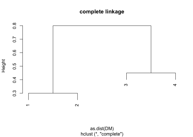
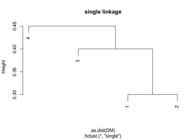
DM <- matrix(data = c(0, 0.3, 0.4, 0.7, 0.3, 0, 0.5, 0.8, 0.4, 0.5, 0, 0.45, 0.7, 0.8, 0.45, 0), nrow = 4, ncol = 4, byrow = TRUE)

plot(hclust(as.dist(DM), method = "complete"), main = "complete linkage")

plot(hclust(as.dist(DM), method = "single"), main = "single linkage")

Exercise 3

set.seed(0)

# Part (a):
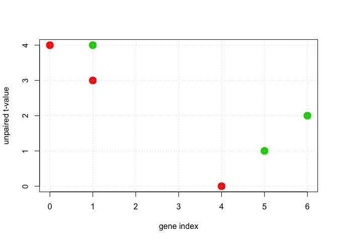
DF <- data.frame(x1 = c(1, 1, 0, 5, 6, 4), x2 = c(4, 3, 4, 1, 2, 0))

n <- dim(DF)[1]
K <- 2

# Part (b): Assign each point to a cluster
labels <- sample(1:K, n, replace = TRUE)

plot(DF$x1, DF$x2, cex = 2, pch = 19, col = (labels + 1), xlab = "gene index", ylab = "unpaired t-value")
grid()

while (TRUE) {

    # Part (c): Compute the centroids of each cluster
    cents <- matrix(nrow = K, ncol = 2)
    for (l in 1:K) {
        samps <- labels == l
        cents[l, ] <- apply(DF[samps, ], 2, mean)
    }

    # Part (d): Assign each sample to the centroid it is closest too:
    new_labels <- rep(NA, n)
    for (si in 1:n) {
        smallest_norm <- +Inf
        for (l in 1:K) {
            nm <- norm(as.matrix(DF[si, ] - cents[l, ]), type = "2")
            if (nm < smallest_norm) {
                smallest_norm <- nm
                new_labels[si] <- l
            }
        }
    }

    # Part (e): Repeat until labels stop changing:
    if (sum(new_labels == labels) == n) {
        break
    } else {
        labels <- new_labels
    }
}

# Part (f): Plot the updated cluster labels
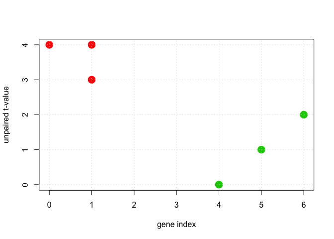
plot(DF$x1, DF$x2, cex = 2, pch = 19, col = (labels + 1), xlab = "gene index", ylab = "unpaired t-value")
grid()

Exercise 7

set.seed(0)

# Scale each observation (not the features):
USA_scaled <- t(scale(t(USArrests)))

# The correlation of each sample with the other samples:
Rij <- cor(t(USA_scaled))  # -1 <= Rij <= +1 
OneMinusRij <- 1 - Rij  # 0 <= 1-Rij <= +2 
X <- OneMinusRij[lower.tri(OneMinusRij)]

D <- as.matrix(dist(USA_scaled)^2)
Y <- D[lower.tri(D)]

plot(X, Y)

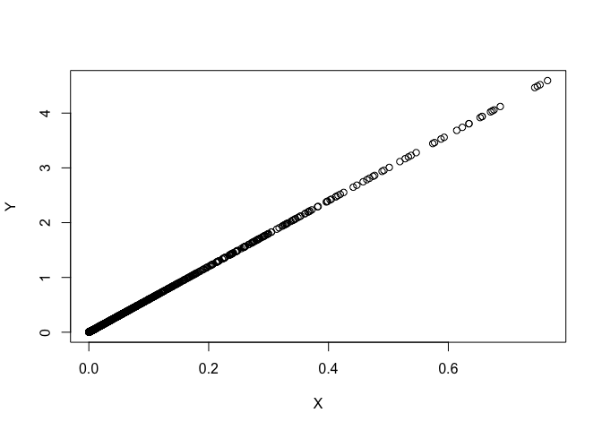
summary(X/Y)

##    Min. 1st Qu.  Median    Mean 3rd Qu.    Max. 
##  0.1667  0.1667  0.1667  0.1667  0.1667  0.1667

Exercise 8

set.seed(0)

pr.out <- prcomp(USArrests, scale = TRUE)

# Using the output from prcomp:
pr.var <- pr.out$sdev^2
pve_1 <- pr.var/sum(pr.var)

# Apply Equation 10.8 directly:
USArrests_scaled <- scale(USArrests)
denom <- sum(apply(USArrests_scaled^2, 2, sum))

Phi <- pr.out$rotation
USArrests_projected <- USArrests_scaled %*% Phi  # this is the same as pr.out$x

numer <- apply(pr.out$x^2, 2, sum)
pve_2 <- numer/denom

print(pve_1)

## [1] 0.62006039 0.24744129 0.08914080 0.04335752

print(pve_2)

##        PC1        PC2        PC3        PC4 
## 0.62006039 0.24744129 0.08914080 0.04335752

print(pve_1 - pve_2)

##           PC1           PC2           PC3           PC4 
## -1.110223e-16 -2.498002e-16 -4.163336e-17  0.000000e+00

Exercise 9

set.seed(0)

# Part (a-b):
hclust.complete <- hclust(dist(USArrests), method = "complete")

plot(hclust.complete, xlab = "", sub = "", cex = 0.9)

# cutree( hclust.complete, h=150 ) # height we cut at
ct <- cutree(hclust.complete, k = 3)  # number of clusters to cut into

# Print which states go into each cluster:
for (k in 1:3) {
    print(k)
    print(rownames(USArrests)[ct == k])
}

## [1] 1
##  [1] "Alabama"        "Alaska"         "Arizona"        "California"    
##  [5] "Delaware"       "Florida"        "Illinois"       "Louisiana"     
##  [9] "Maryland"       "Michigan"       "Mississippi"    "Nevada"        
## [13] "New Mexico"     "New York"       "North Carolina" "South Carolina"
## [1] 2
##  [1] "Arkansas"      "Colorado"      "Georgia"       "Massachusetts"
##  [5] "Missouri"      "New Jersey"    "Oklahoma"      "Oregon"       
##  [9] "Rhode Island"  "Tennessee"     "Texas"         "Virginia"     
## [13] "Washington"    "Wyoming"      
## [1] 3
##  [1] "Connecticut"   "Hawaii"        "Idaho"         "Indiana"      
##  [5] "Iowa"          "Kansas"        "Kentucky"      "Maine"        
##  [9] "Minnesota"     "Montana"       "Nebraska"      "New Hampshire"
## [13] "North Dakota"  "Ohio"          "Pennsylvania"  "South Dakota" 
## [17] "Utah"          "Vermont"       "West Virginia" "Wisconsin"

# Part (c-d):
hclust.complete.scale <- hclust(dist(scale(USArrests, center = FALSE)), method = "complete")

plot(hclust.complete.scale, xlab = "", sub = "", cex = 0.9)

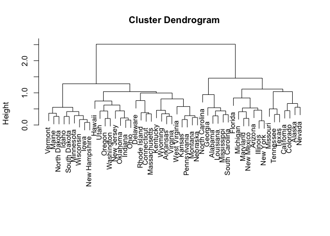
ct <- cutree(hclust.complete.scale, k = 3)  # number of clusters to cut into

# Print which states go into each cluster in this case:
for (k in 1:3) {
    print(k)
    print(rownames(USArrests)[ct == k])
}

## [1] 1
## [1] "Alabama"        "Georgia"        "Louisiana"      "Mississippi"   
## [5] "North Carolina" "South Carolina"
## [1] 2
##  [1] "Alaska"     "Arizona"    "California" "Colorado"   "Florida"   
##  [6] "Illinois"   "Maryland"   "Michigan"   "Missouri"   "Nevada"    
## [11] "New Mexico" "New York"   "Tennessee"  "Texas"     
## [1] 3
##  [1] "Arkansas"      "Connecticut"   "Delaware"      "Hawaii"       
##  [5] "Idaho"         "Indiana"       "Iowa"          "Kansas"       
##  [9] "Kentucky"      "Maine"         "Massachusetts" "Minnesota"    
## [13] "Montana"       "Nebraska"      "New Hampshire" "New Jersey"   
## [17] "North Dakota"  "Ohio"          "Oklahoma"      "Oregon"       
## [21] "Pennsylvania"  "Rhode Island"  "South Dakota"  "Utah"         
## [25] "Vermont"       "Virginia"      "Washington"    "West Virginia"
## [29] "Wisconsin"     "Wyoming"