- Introduction
- 1. Chapter 2. Statistical Learning
- 2. Chapter 3. Linear Regression
- 3. Chapter 4. Classification
- 4. Chapter 5. Resampling Methods
- 5. Chapter 6. Linear Model Selection and Regularization
- 6. Chapter 7. Moving Beyond Linearity
- 7. Chapter 8. Tree-Based Methods
- 8. Chapter 9. Support Vector Machines
- 9. Chapter 10. Unsupervised Learning
- 10. References
- Published with GitBook
4.6 Lab: Logistic Regression, LDA, QDA, and KNN
4.6.1 The Stock Market Data
Start by loading that ISLR package and attach to the Smarket dataset that we will be using throughtout this exercise.
library(ISLR)
attach(Smarket)
names(Smarket)
## [1] "Year"      "Lag1"      "Lag2"      "Lag3"      "Lag4"      "Lag5"
## [7] "Volume"    "Today"     "Direction"
pairs(Smarket)
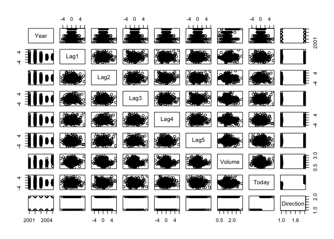
The cor() function is used to show a matrix of all pairwise correlations among the predictors in the Smarket dataset.
cor(Smarket[, -9])
##              Year         Lag1         Lag2         Lag3         Lag4
## Year   1.00000000  0.029699649  0.030596422  0.033194581  0.035688718
## Lag1   0.02969965  1.000000000 -0.026294328 -0.010803402 -0.002985911
## Lag2   0.03059642 -0.026294328  1.000000000 -0.025896670 -0.010853533
## Lag3   0.03319458 -0.010803402 -0.025896670  1.000000000 -0.024051036
## Lag4   0.03568872 -0.002985911 -0.010853533 -0.024051036  1.000000000
## Lag5   0.02978799 -0.005674606 -0.003557949 -0.018808338 -0.027083641
## Volume 0.53900647  0.040909908 -0.043383215 -0.041823686 -0.048414246
## Today  0.03009523 -0.026155045 -0.010250033 -0.002447647 -0.006899527
##                Lag5      Volume        Today
## Year    0.029787995  0.53900647  0.030095229
## Lag1   -0.005674606  0.04090991 -0.026155045
## Lag2   -0.003557949 -0.04338321 -0.010250033
## Lag3   -0.018808338 -0.04182369 -0.002447647
## Lag4   -0.027083641 -0.04841425 -0.006899527
## Lag5    1.000000000 -0.02200231 -0.034860083
## Volume -0.022002315  1.00000000  0.014591823
## Today  -0.034860083  0.01459182  1.000000000
Use the plot() function to produce a scatter plot or the variable Volume.
plot(Volume)

4.6.2 Logistic Regression
The glm() function can be used to fit a logistic regression model by specifying family=binomial.
glm.fit <- glm(Direction ~ Lag1 + Lag2 + Lag3 + Lag4 + Lag5 + Volume, data = Smarket, family = binomial)
summary(glm.fit)
##
## Call:
## glm(formula = Direction ~ Lag1 + Lag2 + Lag3 + Lag4 + Lag5 +
##     Volume, family = binomial, data = Smarket)
##
## Deviance Residuals:
##    Min      1Q  Median      3Q     Max
## -1.446  -1.203   1.065   1.145   1.326
##
## Coefficients:
##              Estimate Std. Error z value Pr(>|z|)
## (Intercept) -0.126000   0.240736  -0.523    0.601
## Lag1        -0.073074   0.050167  -1.457    0.145
## Lag2        -0.042301   0.050086  -0.845    0.398
## Lag3         0.011085   0.049939   0.222    0.824
## Lag4         0.009359   0.049974   0.187    0.851
## Lag5         0.010313   0.049511   0.208    0.835
## Volume       0.135441   0.158360   0.855    0.392
##
## (Dispersion parameter for binomial family taken to be 1)
##
##     Null deviance: 1731.2  on 1249  degrees of freedom
## Residual deviance: 1727.6  on 1243  degrees of freedom
## AIC: 1741.6
##
## Number of Fisher Scoring iterations: 3
Similar to linear models estimated with the lm(), the logistic regression model fitted with glm() can be examined with the summary() and coef()
coef(glm.fit)
##  (Intercept)         Lag1         Lag2         Lag3         Lag4
## -0.126000257 -0.073073746 -0.042301344  0.011085108  0.009358938
##         Lag5       Volume
##  0.010313068  0.135440659
summary(glm.fit)$coef
##                 Estimate Std. Error    z value  Pr(>|z|)
## (Intercept) -0.126000257 0.24073574 -0.5233966 0.6006983
## Lag1        -0.073073746 0.05016739 -1.4565986 0.1452272
## Lag2        -0.042301344 0.05008605 -0.8445733 0.3983491
## Lag3         0.011085108 0.04993854  0.2219750 0.8243333
## Lag4         0.009358938 0.04997413  0.1872757 0.8514445
## Lag5         0.010313068 0.04951146  0.2082966 0.8349974
## Volume       0.135440659 0.15835970  0.8552723 0.3924004
summary(glm.fit)$coef[, 4]
## (Intercept)        Lag1        Lag2        Lag3        Lag4        Lag5
##   0.6006983   0.1452272   0.3983491   0.8243333   0.8514445   0.8349974
##      Volume
##   0.3924004
The predict() function is used similary to generate predictions for the response variable.
glm.probs <- predict(glm.fit, type = "response")
glm.probs[1:10]
##         1         2         3         4         5         6         7
## 0.5070841 0.4814679 0.4811388 0.5152224 0.5107812 0.5069565 0.4926509
##         8         9        10
## 0.5092292 0.5176135 0.4888378
Use the contrasts() function to see the dummy variables generated for values in the categorical variable Direction.
contrasts(Direction)
##      Up
## Down  0
## Up    1
Next we convert the predicted probabilities to either "Up" or "Down" based on whether the probability is less than or greater than 0.5.
glm.pred <- rep("Down", 1250)
glm.pred[glm.probs > 0.5] <- "Up"
We can generate a confusion matrix between the predicted direction and the actual direction from the variable Direction using the table() function.
table(glm.pred, Direction)
##         Direction
## glm.pred Down  Up
##     Down  145 141
##     Up    457 507
mean(glm.pred == Direction)
## [1] 0.5216
We then divide our dataset into training set and validation set. The training set will include observations from 2001-2004 and the validation set from the year 2005.
train <- (Year < 2005)
Smarket.2005= Smarket [! train ,]
dim(Smarket.2005)
## [1] 252 9
Direction.2005=Direction[!train]
We can run the loggistic regression again using glm() but this time restricting our training set to obervations in the subset train.
glm.fit <- glm(Direction ~ Lag1 + Lag2 + Lag3 + Lag4 + Lag5 + Volume, data = Smarket, family = binomial, subset = train)
glm.probs <- predict(glm.fit, Smarket.2005, type = "response")
Next we compare the predictions for 2005 based on the model generated from our train subset.
glm.pred <- rep("Down", 252)
glm.pred[glm.probs > 0.5] <- "Up"
table(glm.pred, Direction.2005)
##         Direction.2005
## glm.pred Down Up
##     Down   77 97
##     Up     34 44
mean(glm.pred == Direction.2005)
## [1] 0.4801587
mean(glm.pred != Direction.2005)
## [1] 0.5198413
To improve the preditive performance, we can restrict the predictor variables to only those with the strongest relationship to the response variable. In this case, we limit the variables to Lag1 and Lag2.
glm.fit <- glm(Direction ~ Lag1 + Lag2, data = Smarket, family = binomial, subset = train)
glm.probs <- predict(glm.fit, Smarket.2005, type = "response")
glm.pred <- rep("Down", 252)
glm.pred[glm.probs > 0.5] <- "Up"
table(glm.pred, Direction.2005)
##         Direction.2005
## glm.pred Down  Up
##     Down   35  35
##     Up     76 106
mean(glm.pred == Direction.2005)
## [1] 0.5595238
predict(glm.fit,newdata=data.frame(Lag1=c(1.2,1.5), Lag2=c(1.1,-0.8)),type="response")
##         1         2
## 0.4791462 0.4960939
4.6.3 Linear Discriminant Analysis
Let's first load the MASS package so we can train an LDA model with the lda() function.
library(MASS)
lda.fit <- lda(Direction ~ Lag1 + Lag2, data = Smarket, subset = train)
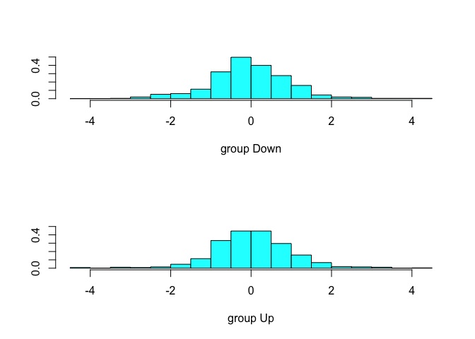
plot(lda.fit)
The preditc() function for an LDA model returns a list of three elements representing the predicted class, the posterior probabilities and the linear discriminants as shown below.
lda.pred <- predict(lda.fit, Smarket.2005)
names(lda.pred)
## [1] "class" "posterior" "x"
We can compare the predicted class with the predicted directed obtained from logistic regression in the previous section and stored in the vector Direction.2005.
lda.class <- lda.pred$class
table(lda.class, Direction.2005)
##          Direction.2005
## lda.class Down  Up
##      Down   35  35
##      Up     76 106
mean(lda.class == Direction.2005)
## [1] 0.5595238
sum(lda.pred$posterior[, 1] >= 0.5)
## [1] 70
sum(lda.pred$posterior[, 1] < 0.5)
## [1] 182
We can inspect the posterior probabilities of the LDA model from the posterior vector of the fitted model.
lda.pred$posterior[1:20, 1]
##       999      1000      1001      1002      1003      1004      1005
## 0.4901792 0.4792185 0.4668185 0.4740011 0.4927877 0.4938562 0.4951016
##      1006      1007      1008      1009      1010      1011      1012
## 0.4872861 0.4907013 0.4844026 0.4906963 0.5119988 0.4895152 0.4706761
##      1013      1014      1015      1016      1017      1018
## 0.4744593 0.4799583 0.4935775 0.5030894 0.4978806 0.4886331
lda.class[1:20]
##  [1] Up   Up   Up   Up   Up   Up   Up   Up   Up   Up   Up   Down Up   Up
## [15] Up   Up   Up   Down Up   Up
## Levels: Down Up
We can also set the posterior probabilities to different thresholds for making predictions.
sum(lda.pred$posterior[, 1] > 0.9)
## [1] 0
4.6.4 Quadratic Discriminant Analysis
In addition to Linear Discriminant Analysis (LDA), the MASS package also offers a Quadratic Discriminant Analysis (LDA) model that we can fit with the qda() function.
qda.fit <- qda(Direction ~ Lag1 + Lag2, data = Smarket, subset = train)
qda.fit
## Call:
## qda(Direction ~ Lag1 + Lag2, data = Smarket, subset = train)
##
## Prior probabilities of groups:
##     Down       Up
## 0.491984 0.508016
##
## Group means:
##             Lag1        Lag2
## Down  0.04279022  0.03389409
## Up   -0.03954635 -0.03132544
We can make predictions using predict() just as we did for an LDA model and compare them to the results from the logistic regression.
qda.class <- predict(qda.fit, Smarket.2005)$class
table(qda.class, Direction.2005)
##          Direction.2005
## qda.class Down  Up
##      Down   30  20
##      Up     81 121
mean(qda.class == Direction.2005)
## [1] 0.5992063
4.6.5 K-Nearest Neighbors
The class package offers a number of classification algorithms including K-Nearest Neighbors. Before we can run the KNN algorithm, we need to split our dataset into training and test subsets. After splitting the dataset, the cbind() is used to bind the Lag1 and Lag2 variables into a matrix for each subset.
library(class)
train.X <- cbind(Lag1, Lag2)[train, ]
test.X <- cbind(Lag1, Lag2)[!train, ]
train.Direction <- Direction[train]
We initialize the random number generator with set.seed() to ensure that repeated runs produce consistent results and then use knn() to make predictions about the market direction in 2005.
set.seed(1)
knn.pred <- knn(train.X, test.X, train.Direction, k = 1)
table(knn.pred, Direction.2005)
##         Direction.2005
## knn.pred Down Up
##     Down   43 58
##     Up     68 83
(83 + 43)/252
## [1] 0.5
We can repeat the fit with K = 3.
knn.pred <- knn(train.X, test.X, train.Direction, k = 3)
table(knn.pred, Direction.2005)
##         Direction.2005
## knn.pred Down Up
##     Down   48 54
##     Up     63 87
mean(knn.pred == Direction.2005)
## [1] 0.5357143
4.6.6 An Application to Caravan Insurance Data
We first use the attach() function to make the Caravan dataset available to us.
attach(Caravan)
Lets explore the dataset with the dim() and summary() functions.
dim(Caravan)
## [1] 5822 86
summary(Purchase)
##   No  Yes
## 5474  348
348/5822
## [1] 0.05977327
We use the scale() function to scale the dataset with a mean of zero and standard deviation of one.
standardized.X <- scale(Caravan[, -86])
var(Caravan[, 1])
## [1] 165.0378
var(Caravan[, 2])
## [1] 0.1647078
var(standardized.X[, 1])
## [1] 1
var(standardized.X[, 2])
## [1] 1
We use the producedure described in the previous section of splitting the dataset into training and test sets and making prediction about the response variable Purchase using a KNN model.
test <- 1:1000
train.X <- standardized.X[-test, ]
test.X <- standardized.X[test, ]
train.Y <- Purchase[-test]
test.Y <- Purchase[test]
set.seed(1)
knn.pred <- knn(train.X, test.X, train.Y, k = 1)
mean(test.Y != knn.pred)
## [1] 0.118
mean(test.Y != "No")
## [1] 0.059
table(knn.pred, test.Y)
##         test.Y
## knn.pred  No Yes
##      No  873  50
##      Yes  68   9
9/(68 + 9)
## [1] 0.1168831
We can repeat this process with different values of K, for example, K = 3 and K = 5.
knn.pred <- knn(train.X, test.X, train.Y, k = 3)
table(knn.pred, test.Y)
##         test.Y
## knn.pred  No Yes
##      No  920  54
##      Yes  21   5
5/26
## [1] 0.1923077
knn.pred <- knn(train.X, test.X, train.Y, k = 5)
table(knn.pred, test.Y)
##         test.Y
## knn.pred  No Yes
##      No  930  55
##      Yes  11   4
4/15
## [1] 0.2666667
Finally, we compare the KNN model with a logistic regression using glm() and family = binomial.
glm.fit <- glm(Purchase ~ ., data = Caravan, family = binomial, subset = -test)
## Warning: glm.fit: fitted probabilities numerically 0 or 1 occurred
glm.probs <- predict(glm.fit, Caravan[test, ], type = "response")
glm.pred <- rep("No", 1000)
glm.pred[glm.probs > 0.5] <- "Yes"
table(glm.pred, test.Y)
##         test.Y
## glm.pred  No Yes
##      No  934  59
##      Yes   7   0
glm.pred <- rep("No", 1000)
glm.pred[glm.probs > 0.25] <- " Yes"
table(glm.pred, test.Y)
##         test.Y
## glm.pred  No Yes
##      Yes  22  11
##     No   919  48
11/(22 + 11)
## [1] 0.3333333