- Introduction
- 1. Chapter 2. Statistical Learning
- 2. Chapter 3. Linear Regression
- 3. Chapter 4. Classification
- 4. Chapter 5. Resampling Methods
- 5. Chapter 6. Linear Model Selection and Regularization
- 6. Chapter 7. Moving Beyond Linearity
- 7. Chapter 8. Tree-Based Methods
- 8. Chapter 9. Support Vector Machines
- 9. Chapter 10. Unsupervised Learning
- 10. References
- Published with GitBook
3.6 Lab: Linear Regression
3.6.1 Libraries
We use library() to access functionality provided by packages not included in the standard R installation. To install a new package, use the install.packages() function from the command line console.
install.packages("ISLR")
Start by loading that MASS and ISLR packages that we will be using throughtout this exercise
library(MASS)
library(ISLR)
3.6.2 Simple Linear Regression
To access the Boston housing dataset from the MASS package, use the attach() function
attach(Boston)
We can use head() and names() to take a look at the Boston dataset
head(Boston)
##      crim zn indus chas   nox    rm  age    dis rad tax ptratio  black
## 1 0.00632 18  2.31    0 0.538 6.575 65.2 4.0900   1 296    15.3 396.90
## 2 0.02731  0  7.07    0 0.469 6.421 78.9 4.9671   2 242    17.8 396.90
## 3 0.02729  0  7.07    0 0.469 7.185 61.1 4.9671   2 242    17.8 392.83
## 4 0.03237  0  2.18    0 0.458 6.998 45.8 6.0622   3 222    18.7 394.63
## 5 0.06905  0  2.18    0 0.458 7.147 54.2 6.0622   3 222    18.7 396.90
## 6 0.02985  0  2.18    0 0.458 6.430 58.7 6.0622   3 222    18.7 394.12
##   lstat medv
## 1  4.98 24.0
## 2  9.14 21.6
## 3  4.03 34.7
## 4  2.94 33.4
## 5  5.33 36.2
## 6  5.21 28.7
names(Boston)
##  [1] "crim"    "zn"      "indus"   "chas"    "nox"     "rm"      "age"
##  [8] "dis"     "rad"     "tax"     "ptratio" "black"   "lstat"   "medv"
Now, lets start with a simple linear model with lm()
lm.fit <- lm(medv ~ lstat)
Instead of attaching the Boston dataset first, we can also specify it directly in lm().
lm.fit <- lm(medv ~ lstat, data = Boston)
We can examine the fitted model, by simply typing its name.
lm.fit
##
## Call:
## lm(formula = medv ~ lstat, data = Boston)
##
## Coefficients:
## (Intercept)        lstat
##       34.55        -0.95
The names() function lists the names of all variables store in the lm.fit model.
names(lm.fit)
##  [1] "coefficients"  "residuals"     "effects"       "rank"
##  [5] "fitted.values" "assign"        "qr"            "df.residual"
##  [9] "xlevels"       "call"          "terms"         "model"
We can extract the coefficients estimated by lm() using the coef() function, and the confidence interval with the confint() function.
coef(lm.fit)
## (Intercept)       lstat
##  34.5538409  -0.9500494
confint(lm.fit)
##                 2.5 %     97.5 %
## (Intercept) 33.448457 35.6592247
## lstat       -1.026148 -0.8739505
We use the predict() function to obtain prediction interval or confidence intervals for a given value of lstat
predict(lm.fit, data.frame(lstat = (c(5, 10, 15))), interval = "confidence")
##        fit      lwr      upr
## 1 29.80359 29.00741 30.59978
## 2 25.05335 24.47413 25.63256
## 3 20.30310 19.73159 20.87461
predict(lm.fit, data.frame(lstat = (c(5, 10, 15))), interval = "prediction")
##        fit       lwr      upr
## 1 29.80359 17.565675 42.04151
## 2 25.05335 12.827626 37.27907
## 3 20.30310  8.077742 32.52846
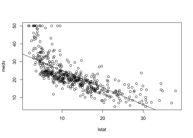
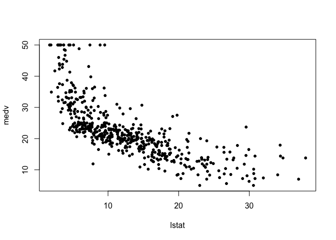
We can plot the variables lstat and medv using the plot() function, and overlay a regression line from our linear model using the abline() function.
plot(lstat, medv)
abline(lm.fit)
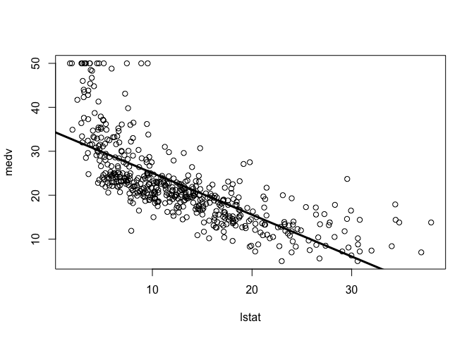
Experiment with different options for abline() by changing the line width and color.
plot(lstat, medv)
abline(lm.fit, lwd = 3)
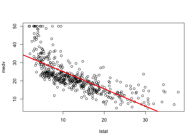
plot(lstat, medv)
abline(lm.fit, lwd = 3, col = "red")
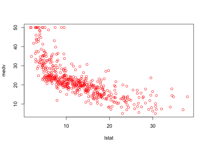
plot(lstat, medv, col = "red")
plot(lstat, medv, pch = 20)
plot(lstat, medv, pch = "+")

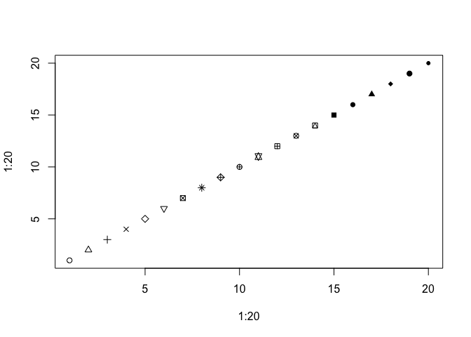
plot(1:20, 1:20, pch = 1:20)
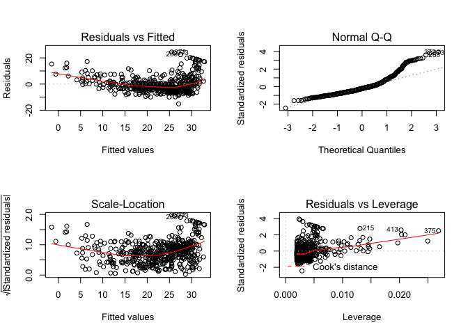
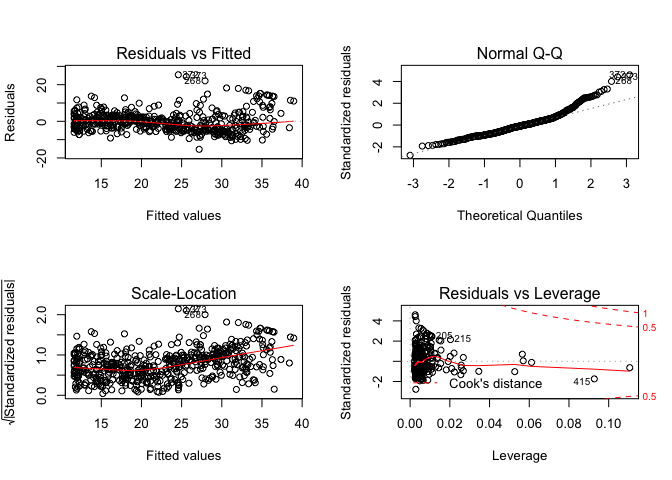
To create a grid of multiple subplots, use the par() function.
par(mfrow = c(2, 2))
plot(lm.fit)
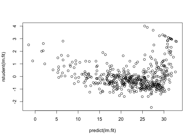
We can extract the residuals and studentized residuals from our linear model using residuals() and rstudent(), and plot them along with the predicted values.
plot(predict(lm.fit), residuals(lm.fit))
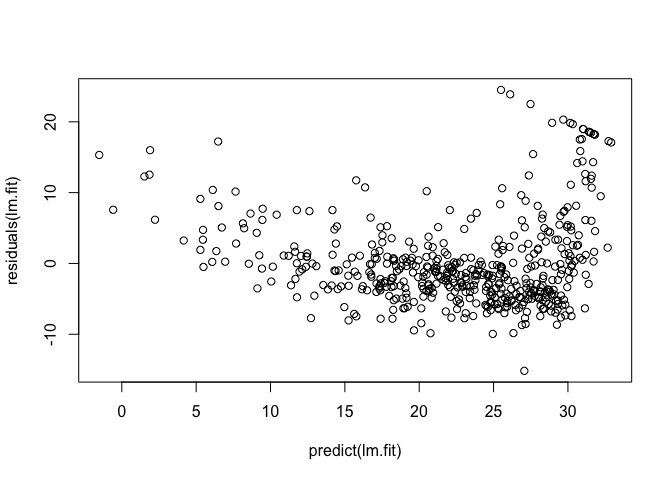
plot(predict(lm.fit), rstudent(lm.fit))
We can compute the influence matrix for the predictors in our fitted model using the hatvalues() function
plot(hatvalues(lm.fit))
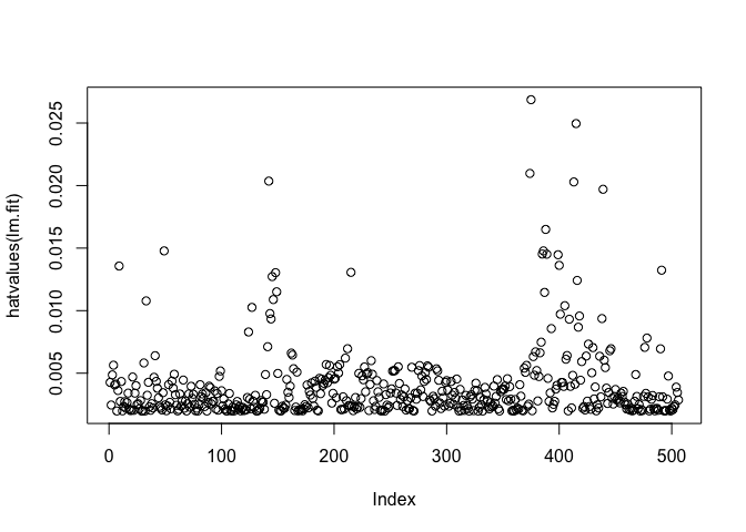
which.max(hatvalues(lm.fit))
## 375
## 375
3.6.3 Multiple Linear Regression
The lm() can be used for fitting multiple regression models as well. In the following example, we include age in addition to lstata as predictors of of our response variable medv.
lm.fit <- lm(medv ~ lstat + age, data = Boston)
summary(lm.fit)
##
## Call:
## lm(formula = medv ~ lstat + age, data = Boston)
##
## Residuals:
##     Min      1Q  Median      3Q     Max
## -15.981  -3.978  -1.283   1.968  23.158
##
## Coefficients:
##             Estimate Std. Error t value Pr(>|t|)
## (Intercept) 33.22276    0.73085  45.458  < 2e-16 ***
## lstat       -1.03207    0.04819 -21.416  < 2e-16 ***
## age          0.03454    0.01223   2.826  0.00491 **
## ---
## Signif. codes:  0 '***' 0.001 '**' 0.01 '*' 0.05 '.' 0.1 ' ' 1
##
## Residual standard error: 6.173 on 503 degrees of freedom
## Multiple R-squared:  0.5513, Adjusted R-squared:  0.5495
## F-statistic:   309 on 2 and 503 DF,  p-value: < 2.2e-16
In a formula, a dot . can be used as a shorthand to include all variables from the Boston dataset as predictors.
lm.fit <- lm(medv ~ ., data = Boston)
summary(lm.fit)
##
## Call:
## lm(formula = medv ~ ., data = Boston)
##
## Residuals:
##     Min      1Q  Median      3Q     Max
## -15.595  -2.730  -0.518   1.777  26.199
##
## Coefficients:
##               Estimate Std. Error t value Pr(>|t|)
## (Intercept)  3.646e+01  5.103e+00   7.144 3.28e-12 ***
## crim        -1.080e-01  3.286e-02  -3.287 0.001087 **
## zn           4.642e-02  1.373e-02   3.382 0.000778 ***
## indus        2.056e-02  6.150e-02   0.334 0.738288
## chas         2.687e+00  8.616e-01   3.118 0.001925 **
## nox         -1.777e+01  3.820e+00  -4.651 4.25e-06 ***
## rm           3.810e+00  4.179e-01   9.116  < 2e-16 ***
## age          6.922e-04  1.321e-02   0.052 0.958229
## dis         -1.476e+00  1.995e-01  -7.398 6.01e-13 ***
## rad          3.060e-01  6.635e-02   4.613 5.07e-06 ***
## tax         -1.233e-02  3.760e-03  -3.280 0.001112 **
## ptratio     -9.527e-01  1.308e-01  -7.283 1.31e-12 ***
## black        9.312e-03  2.686e-03   3.467 0.000573 ***
## lstat       -5.248e-01  5.072e-02 -10.347  < 2e-16 ***
## ---
## Signif. codes:  0 '***' 0.001 '**' 0.01 '*' 0.05 '.' 0.1 ' ' 1
##
## Residual standard error: 4.745 on 492 degrees of freedom
## Multiple R-squared:  0.7406, Adjusted R-squared:  0.7338
## F-statistic: 108.1 on 13 and 492 DF,  p-value: < 2.2e-16
The Variance Inflation Factors (VIF) can be caculated using the vif() function from the Companion to Applied Regression or car package. You can install the car package using install.packages() if it is not already installed.
install.packages("ISLR")
library(car)
vif(lm.fit)
##     crim       zn    indus     chas      nox       rm      age      dis
## 1.792192 2.298758 3.991596 1.073995 4.393720 1.933744 3.100826 3.955945
##      rad      tax  ptratio    black    lstat
## 7.484496 9.008554 1.799084 1.348521 2.941491
To exclude specific variables from the list of predictors, we can use the - notation. In the following example, all variables except age are included in the linear fit model.
lm.fit1 <- lm(medv ~ . - age, data = Boston)
summary(lm.fit1)
##
## Call:
## lm(formula = medv ~ . - age, data = Boston)
##
## Residuals:
##      Min       1Q   Median       3Q      Max
## -15.6054  -2.7313  -0.5188   1.7601  26.2243
##
## Coefficients:
##               Estimate Std. Error t value Pr(>|t|)
## (Intercept)  36.436927   5.080119   7.172 2.72e-12 ***
## crim         -0.108006   0.032832  -3.290 0.001075 **
## zn            0.046334   0.013613   3.404 0.000719 ***
## indus         0.020562   0.061433   0.335 0.737989
## chas          2.689026   0.859598   3.128 0.001863 **
## nox         -17.713540   3.679308  -4.814 1.97e-06 ***
## rm            3.814394   0.408480   9.338  < 2e-16 ***
## dis          -1.478612   0.190611  -7.757 5.03e-14 ***
## rad           0.305786   0.066089   4.627 4.75e-06 ***
## tax          -0.012329   0.003755  -3.283 0.001099 **
## ptratio      -0.952211   0.130294  -7.308 1.10e-12 ***
## black         0.009321   0.002678   3.481 0.000544 ***
## lstat        -0.523852   0.047625 -10.999  < 2e-16 ***
## ---
## Signif. codes:  0 '***' 0.001 '**' 0.01 '*' 0.05 '.' 0.1 ' ' 1
##
## Residual standard error: 4.74 on 493 degrees of freedom
## Multiple R-squared:  0.7406, Adjusted R-squared:  0.7343
## F-statistic: 117.3 on 12 and 493 DF,  p-value: < 2.2e-16
We can also update an existing fit with the update() function and specifiying a new formula.
lm.fit1 <- update(lm.fit, ~. - age)
3.6.4 Interaction Terms
The : and * operators are used to specify interaction terms between variables. The : operator includes just the interaction term between the specified variables as predictor, while the * operator includes the interaction term as well as the variables themselves. In the following example, lstat * age is equivalent to lstat + age + lstat:age
summary(lm(medv ~ lstat * age, data = Boston))
##
## Call:
## lm(formula = medv ~ lstat * age, data = Boston)
##
## Residuals:
##     Min      1Q  Median      3Q     Max
## -15.806  -4.045  -1.333   2.085  27.552
##
## Coefficients:
##               Estimate Std. Error t value Pr(>|t|)
## (Intercept) 36.0885359  1.4698355  24.553  < 2e-16 ***
## lstat       -1.3921168  0.1674555  -8.313 8.78e-16 ***
## age         -0.0007209  0.0198792  -0.036   0.9711
## lstat:age    0.0041560  0.0018518   2.244   0.0252 *
## ---
## Signif. codes:  0 '***' 0.001 '**' 0.01 '*' 0.05 '.' 0.1 ' ' 1
##
## Residual standard error: 6.149 on 502 degrees of freedom
## Multiple R-squared:  0.5557, Adjusted R-squared:  0.5531
## F-statistic: 209.3 on 3 and 502 DF,  p-value: < 2.2e-16
3.6.5 Non-linear Transformations of the Predictors
The lm() function can also be non-linear transformations such as quadratic or cubic terms. Terms in the formula raised to a power with ^ must be wrapped inside a call to I() to prevent interpretation and treated as is.
lm.fit2 <- lm(medv ~ lstat + I(lstat^2))
summary(lm.fit2)
##
## Call:
## lm(formula = medv ~ lstat + I(lstat^2))
##
## Residuals:
##      Min       1Q   Median       3Q      Max
## -15.2834  -3.8313  -0.5295   2.3095  25.4148
##
## Coefficients:
##              Estimate Std. Error t value Pr(>|t|)
## (Intercept) 42.862007   0.872084   49.15   <2e-16 ***
## lstat       -2.332821   0.123803  -18.84   <2e-16 ***
## I(lstat^2)   0.043547   0.003745   11.63   <2e-16 ***
## ---
## Signif. codes:  0 '***' 0.001 '**' 0.01 '*' 0.05 '.' 0.1 ' ' 1
##
## Residual standard error: 5.524 on 503 degrees of freedom
## Multiple R-squared:  0.6407, Adjusted R-squared:  0.6393
## F-statistic: 448.5 on 2 and 503 DF,  p-value: < 2.2e-16
To examine the analysis of variance (ANOVA) for one or more models, we use the anova().
lm.fit <- lm(medv ~ lstat)
anova(lm.fit, lm.fit2)
## Analysis of Variance Table
##
## Model 1: medv ~ lstat
## Model 2: medv ~ lstat + I(lstat^2)
##   Res.Df   RSS Df Sum of Sq     F    Pr(>F)
## 1    504 19472
## 2    503 15347  1    4125.1 135.2 < 2.2e-16 ***
## ---
## Signif. codes:  0 '***' 0.001 '**' 0.01 '*' 0.05 '.' 0.1 ' ' 1
par(mfrow = c(2, 2))
plot(lm.fit2)
lm.fit5 <- lm(medv ~ poly(lstat, 5))
summary(lm.fit5)
##
## Call:
## lm(formula = medv ~ poly(lstat, 5))
##
## Residuals:
##      Min       1Q   Median       3Q      Max
## -13.5433  -3.1039  -0.7052   2.0844  27.1153
##
## Coefficients:
##                  Estimate Std. Error t value Pr(>|t|)
## (Intercept)       22.5328     0.2318  97.197  < 2e-16 ***
## poly(lstat, 5)1 -152.4595     5.2148 -29.236  < 2e-16 ***
## poly(lstat, 5)2   64.2272     5.2148  12.316  < 2e-16 ***
## poly(lstat, 5)3  -27.0511     5.2148  -5.187 3.10e-07 ***
## poly(lstat, 5)4   25.4517     5.2148   4.881 1.42e-06 ***
## poly(lstat, 5)5  -19.2524     5.2148  -3.692 0.000247 ***
## ---
## Signif. codes:  0 '***' 0.001 '**' 0.01 '*' 0.05 '.' 0.1 ' ' 1
##
## Residual standard error: 5.215 on 500 degrees of freedom
## Multiple R-squared:  0.6817, Adjusted R-squared:  0.6785
## F-statistic: 214.2 on 5 and 500 DF,  p-value: < 2.2e-16
In addition to polynomial transformations, the formula in a linear fit model can also include anova() transformations as shown in the following example.
summary(lm(medv ~ log(rm), data = Boston))
##
## Call:
## lm(formula = medv ~ log(rm), data = Boston)
##
## Residuals:
##     Min      1Q  Median      3Q     Max
## -19.487  -2.875  -0.104   2.837  39.816
##
## Coefficients:
##             Estimate Std. Error t value Pr(>|t|)
## (Intercept)  -76.488      5.028  -15.21   <2e-16 ***
## log(rm)       54.055      2.739   19.73   <2e-16 ***
## ---
## Signif. codes:  0 '***' 0.001 '**' 0.01 '*' 0.05 '.' 0.1 ' ' 1
##
## Residual standard error: 6.915 on 504 degrees of freedom
## Multiple R-squared:  0.4358, Adjusted R-squared:  0.4347
## F-statistic: 389.3 on 1 and 504 DF,  p-value: < 2.2e-16
3.6.6 Qualitative Predictors
In this section, we will use the Carseats dataset from the ISLR package. Similar to how we used the Boston dataset, we can make the Carseats dataset available to us with the attach() function.
attach(Carseats, warn.conflicts = FALSE)
head(Carseats)
##   Sales CompPrice Income Advertising Population Price ShelveLoc Age
## 1  9.50       138     73          11        276   120       Bad  42
## 2 11.22       111     48          16        260    83      Good  65
## 3 10.06       113     35          10        269    80    Medium  59
## 4  7.40       117    100           4        466    97    Medium  55
## 5  4.15       141     64           3        340   128       Bad  38
## 6 10.81       124    113          13        501    72       Bad  78
##   Education Urban  US
## 1        17   Yes Yes
## 2        10   Yes Yes
## 3        12   Yes Yes
## 4        14   Yes Yes
## 5        13   Yes  No
## 6        16    No Yes
names(Carseats)
##  [1] "Sales"       "CompPrice"   "Income"      "Advertising" "Population"
##  [6] "Price"       "ShelveLoc"   "Age"         "Education"   "Urban"
## [11] "US"
When dealing with qualitative or categorial variable, R automatically generates dummy variables for us.
lm.fit <- lm(Sales ~ . + Income:Advertising + Price:Age, data = Carseats)
summary(lm.fit)
##
## Call:
## lm(formula = Sales ~ . + Income:Advertising + Price:Age, data = Carseats)
##
## Residuals:
##     Min      1Q  Median      3Q     Max
## -2.9208 -0.7503  0.0177  0.6754  3.3413
##
## Coefficients:
##                      Estimate Std. Error t value Pr(>|t|)
## (Intercept)         6.5755654  1.0087470   6.519 2.22e-10 ***
## CompPrice           0.0929371  0.0041183  22.567  < 2e-16 ***
## Income              0.0108940  0.0026044   4.183 3.57e-05 ***
## Advertising         0.0702462  0.0226091   3.107 0.002030 **
## Population          0.0001592  0.0003679   0.433 0.665330
## Price              -0.1008064  0.0074399 -13.549  < 2e-16 ***
## ShelveLocGood       4.8486762  0.1528378  31.724  < 2e-16 ***
## ShelveLocMedium     1.9532620  0.1257682  15.531  < 2e-16 ***
## Age                -0.0579466  0.0159506  -3.633 0.000318 ***
## Education          -0.0208525  0.0196131  -1.063 0.288361
## UrbanYes            0.1401597  0.1124019   1.247 0.213171
## USYes              -0.1575571  0.1489234  -1.058 0.290729
## Income:Advertising  0.0007510  0.0002784   2.698 0.007290 **
## Price:Age           0.0001068  0.0001333   0.801 0.423812
## ---
## Signif. codes:  0 '***' 0.001 '**' 0.01 '*' 0.05 '.' 0.1 ' ' 1
##
## Residual standard error: 1.011 on 386 degrees of freedom
## Multiple R-squared:  0.8761, Adjusted R-squared:  0.8719
## F-statistic:   210 on 13 and 386 DF,  p-value: < 2.2e-16
To examine the coding for the qualitive variables, we can use the contrasts() function.
contrasts(ShelveLoc)
##        Good Medium
## Bad       0      0
## Good      1      0
## Medium    0      1
3.6.7 Writing Functions
We can define our own functions to wrap a set of R commands in a single call. In the following example, we define a LoadLibraries function that loads the ISLR and MASS packages.
LoadLibraries <- function() {
    library(ISLR)
    library(MASS)
}
The function then simply be called just like any other function supplied with R.
LoadLibraries()