An Introduction to Statistical Learning:

4.7 Exercises

Exercise 10

library("ISLR")
library("MASS")
library("class")

set.seed(0)

# Part (a):
Direction <- Weekly$Direction
Weekly$Direction <- NULL
Weekly$NumericDirection <- as.numeric(Direction)  # Maps Down=>1 and Up=>2
Weekly$NumericDirection[Weekly$NumericDirection == 1] <- -1  # Maps Down=>-1 and Up=>2
Weekly$NumericDirection[Weekly$NumericDirection == 2] <- +1  # Maps Down=>-1 and Up=>+1

# Look at the correlation between the output and the input lags:
Weekly.cor <- cor(Weekly)

# b: logistic regression to predict Direction as a function of 5 lag variables + volume:
Weekly$NumericDirection <- NULL
Weekly$Direction <- Direction

five_lag_model <- glm(Direction ~ Lag1 + Lag2 + Lag3 + Lag4 + Lag5 + Volume, data = Weekly, family = binomial)
summary(five_lag_model)

## 
## Call:
## glm(formula = Direction ~ Lag1 + Lag2 + Lag3 + Lag4 + Lag5 + 
##     Volume, family = binomial, data = Weekly)
## 
## Deviance Residuals: 
##     Min       1Q   Median       3Q      Max  
## -1.6949  -1.2565   0.9913   1.0849   1.4579  
## 
## Coefficients:
##             Estimate Std. Error z value Pr(>|z|)   
## (Intercept)  0.26686    0.08593   3.106   0.0019 **
## Lag1        -0.04127    0.02641  -1.563   0.1181   
## Lag2         0.05844    0.02686   2.175   0.0296 * 
## Lag3        -0.01606    0.02666  -0.602   0.5469   
## Lag4        -0.02779    0.02646  -1.050   0.2937   
## Lag5        -0.01447    0.02638  -0.549   0.5833   
## Volume      -0.02274    0.03690  -0.616   0.5377   
## ---
## Signif. codes:  0 '***' 0.001 '**' 0.01 '*' 0.05 '.' 0.1 ' ' 1
## 
## (Dispersion parameter for binomial family taken to be 1)
## 
##     Null deviance: 1496.2  on 1088  degrees of freedom
## Residual deviance: 1486.4  on 1082  degrees of freedom
## AIC: 1500.4
## 
## Number of Fisher Scoring iterations: 4

contrasts(Weekly$Direction)

##      Up
## Down  0
## Up    1

# c: the confusion matrix:
p_hat <- predict(five_lag_model, newdata = Weekly, type = "response")
y_hat <- rep("Down", length(p_hat))
y_hat[p_hat > 0.5] <- "Up"
CM <- table(predicted = y_hat, truth = Weekly$Direction)
CM

##          truth
## predicted Down  Up
##      Down   54  48
##      Up    430 557

sprintf("LR (all features): overall fraction correct= %10.6f", (CM[1, 1] + CM[2, 2])/sum(CM))

## [1] "LR (all features): overall fraction correct=   0.561065"

# d: logistic regression using only Lag2 as the predictor (since it is the most significant predictor)
Weekly.train <- (Weekly$Year >= 1990) & (Weekly$Year <= 2008)  # our training set 
Weekly.test <- (Weekly$Year >= 2009)  # our testing set 
lag2_model <- glm(Direction ~ Lag2, data = Weekly, family = binomial, subset = Weekly.train)

# CM on test data :
p_hat <- predict(lag2_model, newdata = Weekly[Weekly.test, ], type = "response")
y_hat <- rep("Down", length(p_hat))
y_hat[p_hat > 0.5] <- "Up"
CM <- table(predicted = y_hat, truth = Weekly[Weekly.test, ]$Direction)
CM

##          truth
## predicted Down Up
##      Down    9  5
##      Up     34 56

sprintf("LR (only Lag2): overall fraction correct= %10.6f", (CM[1, 1] + CM[2, 2])/sum(CM))

## [1] "LR (only Lag2): overall fraction correct=   0.625000"

# e: Use LDA
lda.fit <- lda(Direction ~ Lag2, data = Weekly, subset = Weekly.train)

lda.predict <- predict(lda.fit, newdata = Weekly[Weekly.test, ])
CM <- table(predicted = lda.predict$class, truth = Weekly[Weekly.test, ]$Direction)
CM

##          truth
## predicted Down Up
##      Down    9  5
##      Up     34 56

sprintf("LDA (only Lag2): overall fraction correct= %10.6f", (CM[1, 1] + CM[2, 2])/sum(CM))

## [1] "LDA (only Lag2): overall fraction correct=   0.625000"

# f: Use QDA
qda.fit <- qda(Direction ~ Lag2, data = Weekly, subset = Weekly.train)

qda.predict <- predict(qda.fit, newdata = Weekly[Weekly.test, ])
CM <- table(predicted = qda.predict$class, truth = Weekly[Weekly.test, ]$Direction)
CM

##          truth
## predicted Down Up
##      Down    0  0
##      Up     43 61

sprintf("QDA (only Lag2): overall fraction correct= %10.6f", (CM[1, 1] + CM[2, 2])/sum(CM))

## [1] "QDA (only Lag2): overall fraction correct=   0.586538"

# g: KNN
X.train <- data.frame(Lag2 = Weekly[Weekly.train, ]$Lag2)
Y.train <- Weekly[Weekly.train, ]$Direction

X.test <- data.frame(Lag2 = Weekly[Weekly.test, ]$Lag2)

y_hat_k_1 <- knn(X.train, X.test, Y.train, k = 1)

CM <- table(predicted = y_hat_k_1, truth = Weekly[Weekly.test, ]$Direction)
CM

##          truth
## predicted Down Up
##      Down   21 29
##      Up     22 32

sprintf("KNN (k=1): overall fraction correct= %10.6f", (CM[1, 1] + CM[2, 2])/sum(CM))

## [1] "KNN (k=1): overall fraction correct=   0.509615"

y_hat_k_3 <- knn(X.train, X.test, Y.train, k = 3)
CM <- table(predicted = y_hat_k_3, truth = Weekly[Weekly.test, ]$Direction)
CM

##          truth
## predicted Down Up
##      Down   15 19
##      Up     28 42

sprintf("KNN (k=1): overall fraction correct= %10.6f", (CM[1, 1] + CM[2, 2])/sum(CM))

## [1] "KNN (k=1): overall fraction correct=   0.548077"

Exercise 11

attach(Auto)

set.seed(0)

# Part (a):
mpg01 <- rep(0, dim(Auto)[1])  # 0 => less than the median of mpg 
mpg01[Auto$mpg > median(Auto$mpg)] <- 1  # 1 => greater than the median of mpg 

Auto$mpg01 <- mpg01
Auto$mpg <- NULL

# Part (b):
pairs(Auto)

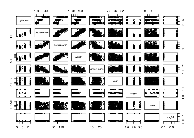
Auto$mpg01 <- as.factor(mpg01)

# Part (c):
n <- dim(Auto)[1]
inds.train <- sample(1:n, 3 * n/4)
Auto.train <- Auto[inds.train, ]
inds.test <- (1:n)[-inds.train]
Auto.test <- Auto[inds.test, ]

# Part (d) Use LDA:
lda.fit <- lda(mpg01 ~ cylinders + displacement + weight, data = Auto.train)

lda.predict <- predict(lda.fit, newdata = Auto.test)
CM <- table(predicted = lda.predict$class, truth = Auto.test$mpg01)
CM

##          truth
## predicted  0  1
##         0 42  1
##         1  5 50

sprintf("LDA: overall fraction correct= %10.6f", (CM[1, 1] + CM[2, 2])/sum(CM))

## [1] "LDA: overall fraction correct=   0.938776"

# Part (e): Use QDA:
qda.fit <- qda(mpg01 ~ cylinders + displacement + weight, data = Auto.train)

qda.predict <- predict(qda.fit, newdata = Auto.test)
CM <- table(predicted = qda.predict$class, truth = Auto.test$mpg01)
CM

##          truth
## predicted  0  1
##         0 44  2
##         1  3 49

sprintf("QDA: overall fraction correct= %10.6f", (CM[1, 1] + CM[2, 2])/sum(CM))

## [1] "QDA: overall fraction correct=   0.948980"

# Part (f): Use Logistic regression:
lr.fit <- glm(mpg01 ~ cylinders + displacement + weight, data = Auto.train, family = binomial)

p_hat <- predict(lr.fit, newdata = Auto.test, type = "response")
y_hat <- rep(0, length(p_hat))
y_hat[p_hat > 0.5] <- 1
CM <- table(predicted = as.factor(y_hat), truth = Auto.test$mpg01)
CM

##          truth
## predicted  0  1
##         0 43  3
##         1  4 48

sprintf("LR (all features): overall fraction correct= %10.6f", (CM[1, 1] + CM[2, 2])/sum(CM))

## [1] "LR (all features): overall fraction correct=   0.928571"

Exercise 12

# Part (a):
Power <- function() {
    print(2^3)
}

# Part (b):
Power2 <- function(x, a) {
    print(x^a)
}

Exercise 13

set.seed(0)

n <- dim(Boston)[1]

# Introduce a variable whether or not the crime rate is above=1 / below=0 the median
Boston$crim01 <- rep(0, n)
Boston$crim01[Boston$crim >= median(Boston$crim)] <- 1
Boston$crim <- NULL

# Look to see what features are most strongly correlated with crim01:
Boston.cor <- cor(Boston)
print(sort(Boston.cor[, "crim01"]))

##         dis          zn       black        medv          rm        chas 
## -0.61634164 -0.43615103 -0.35121093 -0.26301673 -0.15637178  0.07009677 
##     ptratio       lstat       indus         tax         age         rad 
##  0.25356836  0.45326273  0.60326017  0.60874128  0.61393992  0.61978625 
##         nox      crim01 
##  0.72323480  1.00000000

# Split the data set into testing and training parts:
inds.train <- sample(1:n, 3 * n/4)
inds.test <- (1:n)[-inds.train]
Boston.train <- Boston[inds.train, ]
Boston.test <- Boston[inds.test, ]

# Fit several models to the training data
lr_model <- glm(crim01 ~ nox + rad + dis, data = Boston.train, family = binomial)

p_hat <- predict(lr_model, newdata = Boston.test, type = "response")
y_hat <- rep(0, length(p_hat))
y_hat[p_hat > 0.5] <- 1
CM <- table(predicted = y_hat, truth = Boston.test$crim01)
CM

##          truth
## predicted  0  1
##         0 56 15
##         1  4 52

sprintf("LR: overall fraction correct= %10.6f", (CM[1, 1] + CM[2, 2])/sum(CM))

## [1] "LR: overall fraction correct=   0.850394"

lda.fit <- lda(crim01 ~ nox + rad + dis, data = Boston.train)

# Use LDA
lda.fit <- lda(crim01 ~ nox + rad + dis, data = Boston.train)

lda.predict <- predict(lda.fit, newdata = Boston.test)
CM <- table(predicted = lda.predict$class, truth = Boston.test$crim01)
CM

##          truth
## predicted  0  1
##         0 57 21
##         1  3 46

sprintf("LDA: overall fraction correct= %10.6f", (CM[1, 1] + CM[2, 2])/sum(CM))

## [1] "LDA: overall fraction correct=   0.811024"

# f: Use QDA
qda.fit <- qda(crim01 ~ nox + rad + dis, data = Boston.train)

qda.predict <- predict(qda.fit, newdata = Boston.test)
CM <- table(predicted = qda.predict$class, truth = Boston.test$crim01)
CM

##          truth
## predicted  0  1
##         0 58 22
##         1  2 45

sprintf("QDA: overall fraction correct= %10.6f", (CM[1, 1] + CM[2, 2])/sum(CM))

## [1] "QDA: overall fraction correct=   0.811024"

# g: KNN
X.train <- Boston.train
X.train$crim01 <- NULL
Y.train <- Boston.train$crim01

X.test <- Boston.test
X.test$crim01 <- NULL

y_hat_k_1 <- knn(X.train, X.test, Y.train, k = 1)

CM <- table(predicted = y_hat_k_1, truth = Boston.test$crim01)
CM

##          truth
## predicted  0  1
##         0 59  9
##         1  1 58

sprintf("KNN (k=1): overall fraction correct= %10.6f", (CM[1, 1] + CM[2, 2])/sum(CM))

## [1] "KNN (k=1): overall fraction correct=   0.921260"

y_hat_k_3 <- knn(X.train, X.test, Y.train, k = 3)
CM <- table(predicted = y_hat_k_3, truth = Boston.test$crim01)
CM

##          truth
## predicted  0  1
##         0 58 10
##         1  2 57

sprintf("KNN (k=3): overall fraction correct= %10.6f", (CM[1, 1] + CM[2, 2])/sum(CM))

## [1] "KNN (k=3): overall fraction correct=   0.905512"