11 Theme and Title
First, let’s try some of the themes from the ggthemes package
ggplot(northeast, aes(x = Date, y = Home.Value, color = State)) +
  geom_line() +
  theme_stata()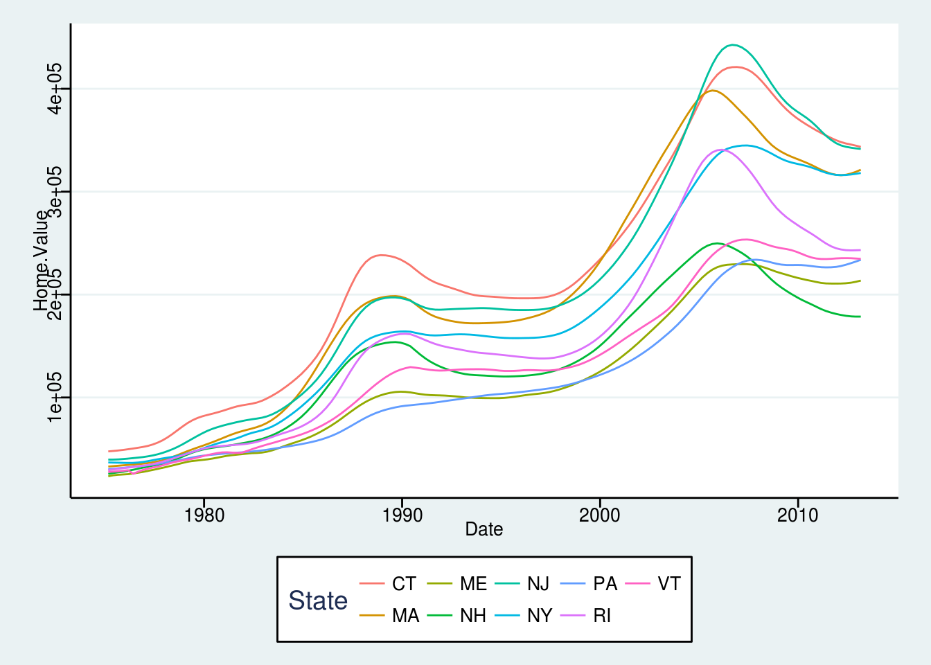
ggplot(northeast, aes(x = Date, y = Home.Value, color = State)) +
  geom_line() +
  theme_economist()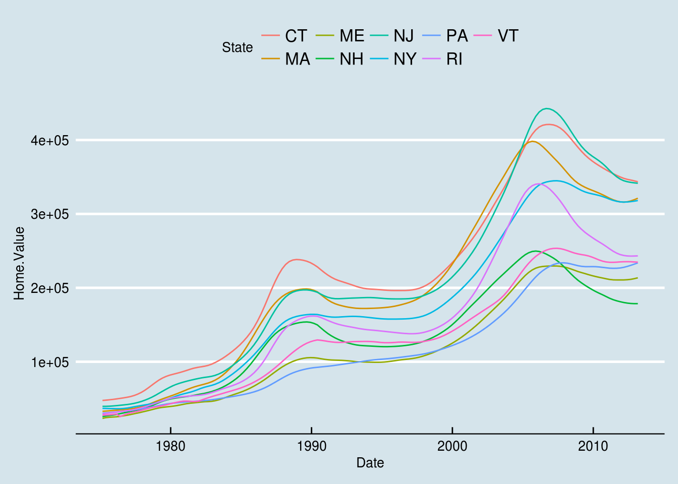
ggplot(northeast, aes(x = Date, y = Home.Value, color = State)) +
  geom_line() +
  theme_wsj()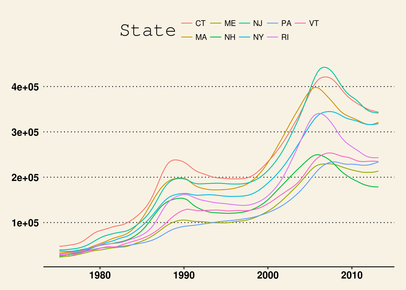
ggplot(northeast, aes(x = Date, y = Home.Value, color = State)) +
  geom_line() +
  theme_solarized()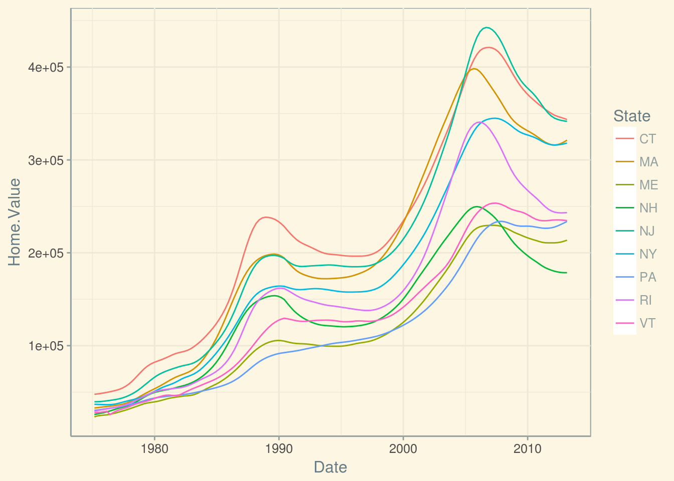
ggplot(northeast, aes(x = Date, y = Home.Value, color = State)) +
  geom_line() +
  theme_fivethirtyeight()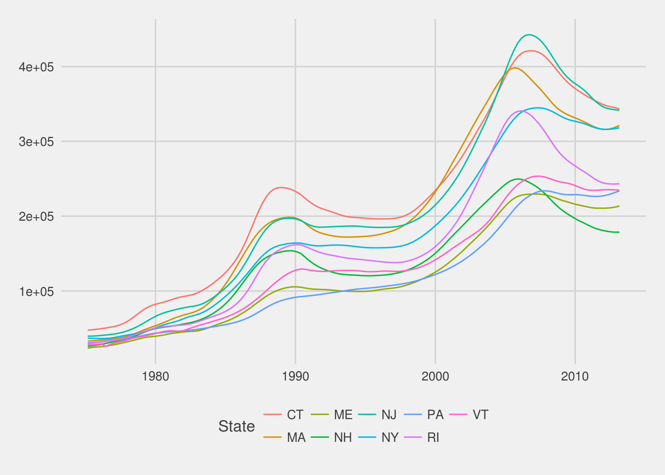
We can also have complete control over the theme by customizing each element ourselves. Let’s start with theme_minimal()
ggplot(northeast, aes(x = Date, y = Home.Value, color = State)) +
  geom_line() +
  theme_minimal()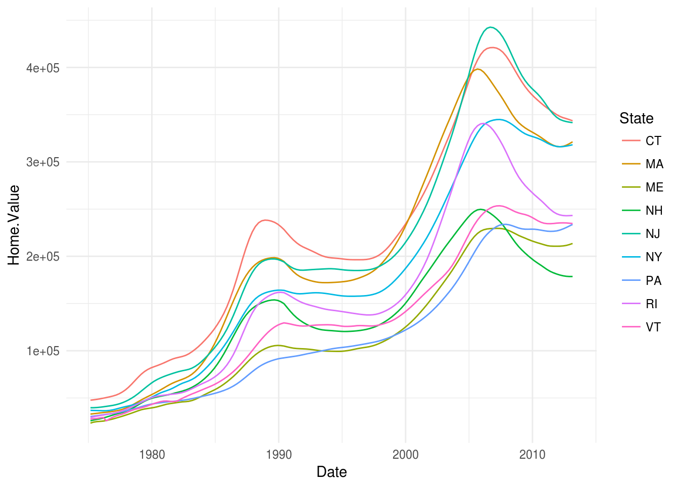
Now remove the minor grid lines
ggplot(northeast, aes(x = Date, y = Home.Value, color = State)) +
  geom_line() +
  theme_minimal() +
  theme(
    panel.grid.minor = element_blank()
  )
Next, we change the y-axis label
ggplot(northeast, aes(x = Date, y = Home.Value, color = State)) +
  geom_line() +
  theme_minimal() +
  theme(
    panel.grid.minor = element_blank()
  ) +
  ylab("Home Value (US$)")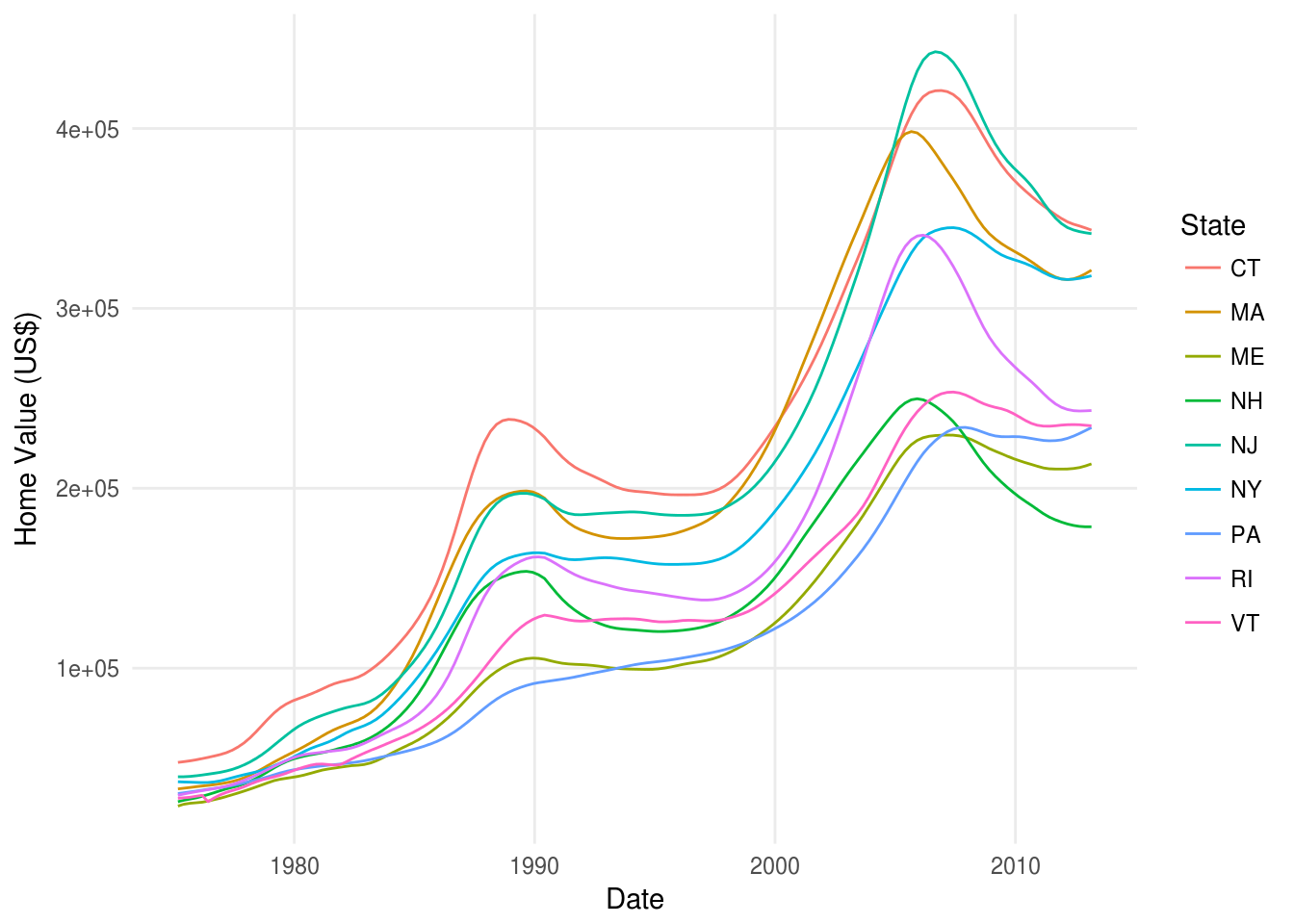
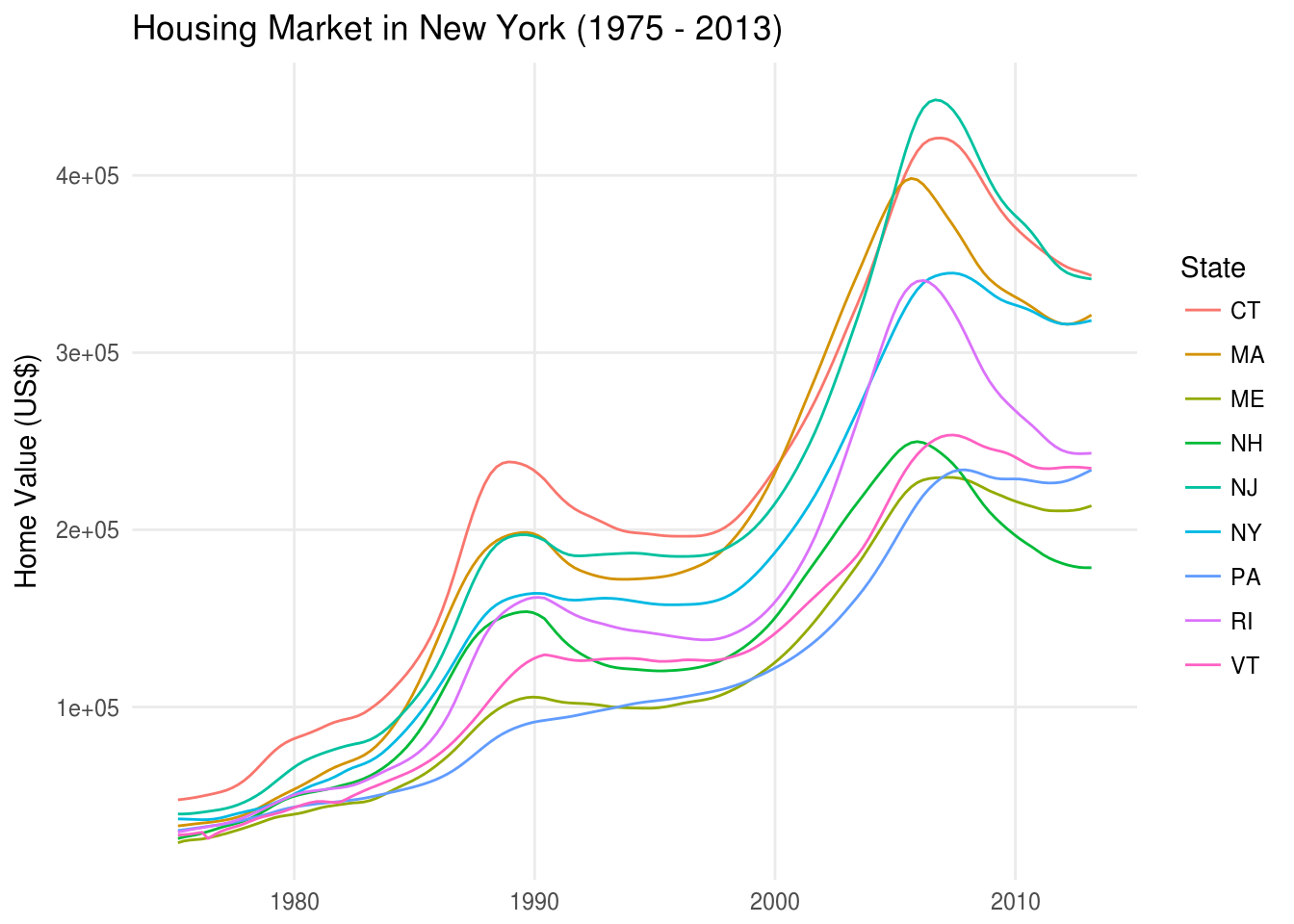
Then remove the x-axis title since the year is self explanatory
ggplot(northeast, aes(x = Date, y = Home.Value, color = State)) +
  geom_line() +
  theme_minimal() +
  theme(
    axis.title.x = element_blank(),
    panel.grid.minor = element_blank()
  ) +
  ylab("Home Value (US$)")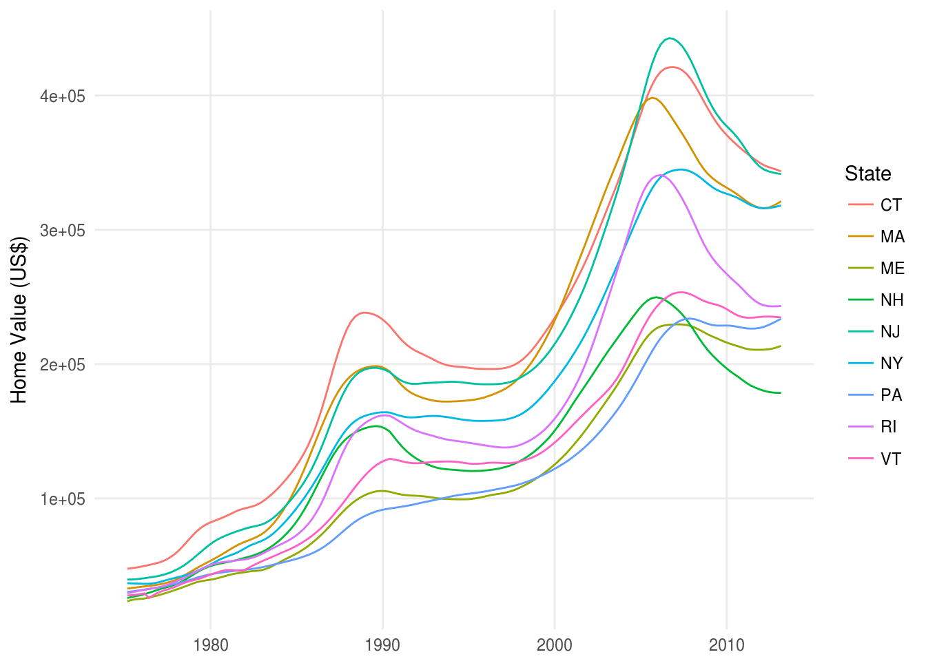
Finally, we can add a title to our plot
ggplot(northeast, aes(x = Date, y = Home.Value, color = State)) +
  geom_line() +
  theme_minimal() +
  theme(
    axis.title.x = element_blank(),
    panel.grid.minor = element_blank()
  ) +
  ylab("Home Value (US$)") +
  ggtitle("Housing Market in New York (1975 - 2013)")