3 Panel Data Models
Panel data are datasets in which a set of units (for example people) are observed for several time periods.
If experimental data are not available, then the use of panel data is one important approach to reduce the problem of omitted variable bias.
There are many empirical research areas where results that are not based on panel data are no longer taken seriously.
3.1 Fixed Effects Model
The fixed effects model is simply a variation on the linear regression model.
Its key advantage is that it enables us to control for all variables that vary over the cross-sectional units but are constant over time.
3.1.1 Example: Traffic Fatalities and Beer Tax
Dataset from Stock & Watson (Ch.10), covers state traffic fatality data available for 48 states observed over seven years (from 1982 to 1988), for a total of 336 observations.
| state | year | mrall | beertax | mlda | jaild | vmiles | unrate | perinc |
|---|---|---|---|---|---|---|---|---|
| AL | 1982 | 0.0002128 | 1.5393795 | 19.00 | 0 | 7233.887 | 14.4 | 10544.15 |
| AL | 1983 | 0.0002348 | 1.7889907 | 19.00 | 0 | 7836.348 | 13.7 | 10732.80 |
| AL | 1984 | 0.0002336 | 1.7142856 | 19.00 | 0 | 8262.990 | 11.1 | 11108.79 |
| AL | 1985 | 0.0002193 | 1.6525424 | 19.67 | 0 | 8726.917 | 8.9 | 11332.63 |
| AL | 1986 | 0.0002669 | 1.6099070 | 21.00 | 0 | 8952.854 | 9.8 | 11661.51 |
| AL | 1987 | 0.0002719 | 1.5599999 | 21.00 | 0 | 9166.302 | 7.8 | 11944.00 |
| AL | 1988 | 0.0002494 | 1.5014436 | 21.00 | 0 | 9674.323 | 7.2 | 12368.62 |
| AZ | 1982 | 0.0002499 | 0.2147971 | 19.00 | 1 | 6810.157 | 9.9 | 12309.07 |
| AZ | 1983 | 0.0002267 | 0.2064220 | 19.00 | 1 | 6587.495 | 9.1 | 12693.81 |
| AZ | 1984 | 0.0002829 | 0.2967033 | 19.00 | 1 | 6709.970 | 5.0 | 13265.93 |
3.2 Assumptions of the Fixed Effects Model
The fixed effects model assumes that the true relationship is:
\[\begin{aligned} y_{i,t} = \beta_0 + \beta_1x_{i,t} + \beta_2z_i + u_{i,t} \end{aligned}\]
where in the S&W example \(y_{i,t}\) would be the number of traffic fatalities and \(x_{i,t}\) the beer tax in state \(i\) in year \(t\).
Note that the variable \(z_i\) does not have a time index and is therefore assumed to be constant over time.
In this example \(z_i\) could be the social attitude towards drunk driving in state \(i\).
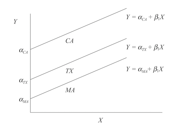
If we define \(\alpha_i = \beta_0 + \beta_2z_i\), then (1) simplifies to
\[\begin{aligned} y_{i,t} = \alpha_i + \beta_1x_{i,t} + u_{i,t} \end{aligned}\]
The graphical interpretation of \(\alpha_i\) is that it is the intercept of the relationship between alcohol taxes and traffic fatalities in state \(i\).
It is straightforward to allow for further variables which are constant over time in (1).
In this case the intercepts \(\alpha_i\) reflect the combined effect of several variables which are constant over time.

3.3 Advantages and Disadvantages
The key advantage of the fixed effects model is that it allows us to control for all time invariant omitted variables.
This is particularly important in the case of variables which are difficult or impossible to observe.
The key disadvantage is that we have to estimate a number of additional parameters.
Furthermore, it will be impossible to estimate the effect of variables which do not (or hardly) vary over time.
3.4 Time Fixed Effects
The basic fixed effects model only prevents omitted variable bias from variables that do not change over time.
However, panel data allow us to control also for omitted variable bias from one other type of omitted variable.
In the traffic fatalities example technical progress could be an important determinant of the number of deaths and could also be correlated with alcohol taxes.
At the same time this variable probably affects all states in the same way (i.e. does not vary across states).
3.5 Time and Unit Fixed Effects
In most applications we use both unit and time fixed effects at the same time.
This model is sometimes referred to as the “twoway fixed effects” model.
In the literature the cross-sectional fixed effects are referred to as “fixed effects”, “state (fixed) effects”, “firm (fixed) effects” or “person (fixed) effects”.
Similarly, time fixed effects are often referred to as “time effects”.