2 Activity
library(plyr)
library(cshapes)
library(countrycode)
library(tidyverse)
library(lubridate)
library(broom)
library(yaml)
library(ggrepel)
2.1 Loading Dataset
Load Phoenix events and few other things we need for plotting.
source('R/phoenix.R')

config <- yaml.load_file("config.yml")
events <- phoenix_load(config, "2017-01-01")
country_centroids <- read_csv(config$google$centroids)
world_map <- tidy(cshp(as.Date("2016-06-30")), region = "COWCODE")
## Warning: use rgdal::readOGR or sf::st_readFunction for summarizing events. Return value contains a list of nodes and edges reprensenting dyadic events.
get_event_summary <- function(events, centroids, period = 0) {
  events <- events %>%
    filter(Date >= (max(Date) - days(period))) %>%
    filter(SourceActorRole == "GOV" & TargetActorRole == "GOV")

  nodes <- events %>%
    mutate(TargetActorEntity = ifelse(SourceActorEntity == TargetActorEntity, NA, TargetActorEntity)) %>%
    gather(ActorType, ActorEntity, SourceActorEntity, TargetActorEntity) %>%
    filter(!is.na(ActorEntity), !(ActorEntity == "")) %>%
    group_by(ActorEntity) %>%
    summarize(EventCount = n()) %>%
    mutate(CountryCode = countrycode(ActorEntity, "iso3c", "cown"), EventCount) %>%
    select(CountryCode, Country = ActorEntity, EventCount) %>%
    left_join(centroids, by = "Country") %>%
    arrange(desc(EventCount))

  edges <- events %>%
    filter(!is.na(SourceActorEntity), !(SourceActorEntity == ""),
           !is.na(TargetActorEntity), !(TargetActorEntity == ""),
           SourceActorEntity != TargetActorEntity) %>%
    rowwise() %>%
    mutate(Dyad = paste(sort(c(SourceActorEntity, TargetActorEntity)), collapse = "-")) %>%
    ungroup() %>%
    group_by(Dyad) %>%
    summarize(EventCount = n()) %>%
    ungroup() %>%
    separate(Dyad, c("SideA", "SideB"), "-", remove = FALSE) %>%
    mutate(CountryA = countrycode(SideA, "iso3c", "country.name"),
           CountryB = countrycode(SideB, "iso3c", "country.name")) %>%
    left_join(centroids, by = c("SideA" = "Country")) %>%
    select(Dyad, SideA, SideB, CountryA, CountryB, EventCount, SideA_Latitude = Latitude, SideA_Longitude = Longitude) %>%
    left_join(centroids, by = c("SideB" = "Country")) %>%
    select(Dyad, SideA, SideB, CountryA, CountryB, EventCount, SideA_Latitude, SideA_Longitude, SideB_Latitude = Latitude, SideB_Longitude = Longitude) %>%
    arrange(desc(EventCount))

  return(list(nodes = nodes, edges = edges))
}
Function for plotting activity on a map.
plot_activity <- function(map, event_summary) {
  map <- map %>%
    mutate(id = as.numeric(id)) %>%
    left_join(event_summary$nodes, by = c("id" = "CountryCode"))

  ggplot(map) +
    geom_map(map = map, aes(map_id = id, fill = EventCount), color = "gray", size = 0.5) +
    scale_fill_distiller(name = "Event Count", palette = "Blues", direction = 1, na.value = "white") +
    expand_limits(x = map$long, y = map$lat) +
    coord_cartesian() +
    geom_point(aes(x = Longitude, y = Latitude),
               data = event_summary$nodes,
               size = 0.5) +
    geom_curve(aes(x = SideA_Longitude,
                   y = SideA_Latitude,
                   xend = SideB_Longitude,
                   yend = SideB_Latitude),
               data = event_summary$edges,
               size = 0.2,
               alpha = 0.5,
               color = "red") +
    geom_text_repel(aes(x = Longitude, y = Latitude, label = CountryName),
                    data = head(event_summary$nodes, 10),
                    force = 0.1,
                    size = 3,
                    fontface = "bold") +
    theme_minimal() +
    theme(legend.position = "bottom",
          legend.key.width = unit(5, "line"),
          axis.title = element_blank(),
          axis.text = element_blank(),
          panel.grid = element_blank())
}
This function simply formats the top 10 rows from the dataset in a pretty table.
show_top10 <- function(x) {
  x %>%
    head(n = 10) %>%
    knitr::kable()
}
2.2 Most Active on 2017-04-30
event_summary <- get_event_summary(events, country_centroids)
show_top10(select(event_summary$nodes, CountryName, EventCount))| CountryName | EventCount |
|---|---|
| United States | 20 |
| Canada | 12 |
| Mexico | 8 |
| Germany | 6 |
| France | 6 |
| Iran, Islamic Republic of | 6 |
| Russian Federation | 5 |
| China | 4 |
| Ethiopia | 4 |
| Kenya | 4 |
show_top10(select(event_summary$edges, CountryA, CountryB, EventCount))| CountryA | CountryB | EventCount |
|---|---|---|
| Canada | Mexico | 8 |
| Canada | United States of America | 4 |
| Ethiopia | Iran (Islamic Republic of) | 4 |
| France | United States of America | 4 |
| Philippines | United States of America | 4 |
| China | Republic of Korea | 2 |
| China | South Africa | 2 |
| Germany | France | 2 |
| Germany | Russian Federation | 2 |
| Germany | United States of America | 2 |
plot_activity(world_map, event_summary)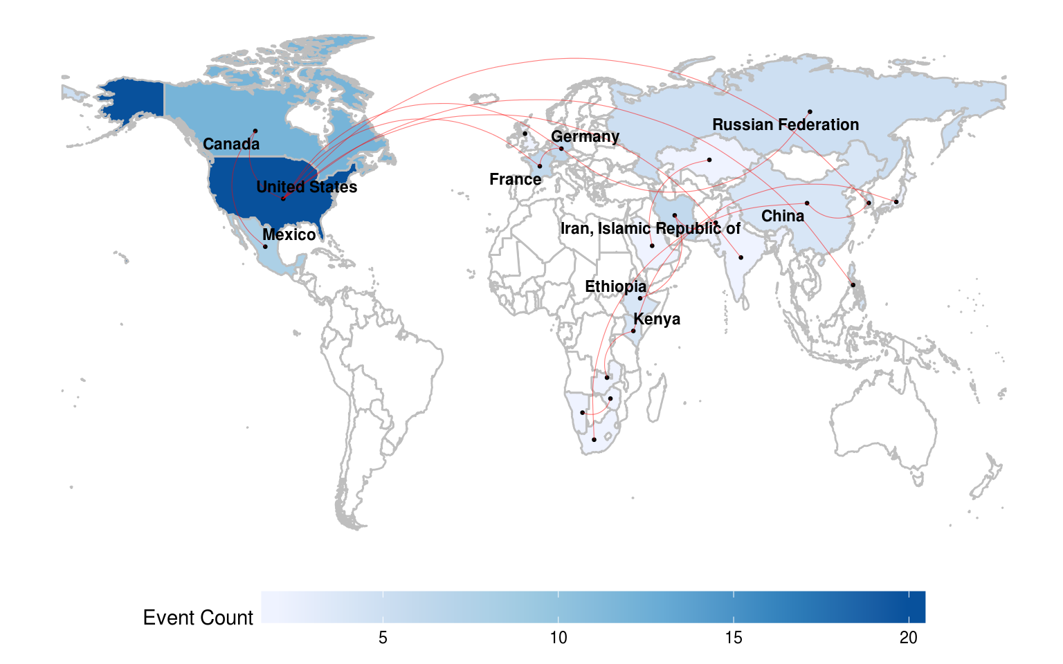
2.3 Most Active in Last 7 Days
event_summary <- get_event_summary(events, country_centroids, period = 7)## Warning in countrycode(c("AFG", "ARG", "AUS", "BEL", "BGD", "BRA", "CAN", : Some values were not matched unambiguously: HKG, IGO, PSE## Warning in countrycode(c("AFG", "ARG", "AUS", "BEL", "BGD", "BGD", "BRA", : Some values were not matched unambiguously: IGOshow_top10(select(event_summary$nodes, CountryName, EventCount))| CountryName | EventCount |
|---|---|
| United States | 325 |
| Russian Federation | 77 |
| China | 74 |
| Japan | 54 |
| Germany | 48 |
| Iran, Islamic Republic of | 45 |
| Canada | 43 |
| Mexico | 43 |
| Israel | 38 |
| Turkey | 36 |
show_top10(select(event_summary$edges, CountryA, CountryB, EventCount))| CountryA | CountryB | EventCount |
|---|---|---|
| Canada | Mexico | 31 |
| Germany | Israel | 28 |
| Japan | Russian Federation | 28 |
| India | United States of America | 26 |
| China | United States of America | 18 |
| Iran (Islamic Republic of) | United States of America | 17 |
| China | Japan | 16 |
| Syrian Arab Republic | United States of America | 16 |
| Egypt | Saudi Arabia | 14 |
| Turkey | United States of America | 14 |
plot_activity(world_map, event_summary)## Warning: Removed 1 rows containing missing values (geom_point).## Warning: Removed 1 rows containing missing values (geom_curve).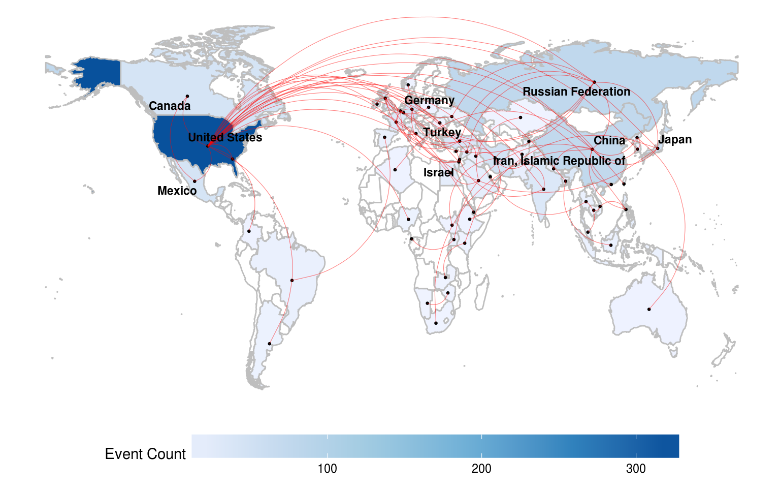
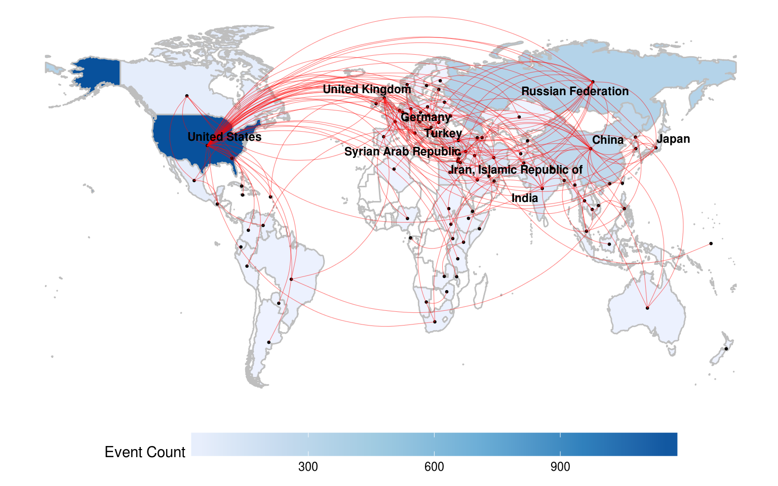
2.4 Most Active in Last 30 Days
event_summary <- get_event_summary(events, country_centroids, period = 30)## Warning in countrycode(c("AFG", "ARE", "ARG", "ARM", "AUS", "AZE", "BEL", : Some values were not matched unambiguously: HKG, IGO, PSE, SRB## Warning in countrycode(c("AFG", "AFG", "AFG", "AFG", "ARE", "ARG", "ARM", : Some values were not matched unambiguously: IGOshow_top10(select(event_summary$nodes, CountryName, EventCount))| CountryName | EventCount |
|---|---|
| United States | 1184 |
| Russian Federation | 346 |
| China | 272 |
| Syrian Arab Republic | 266 |
| Turkey | 161 |
| Germany | 160 |
| United Kingdom | 148 |
| Iran, Islamic Republic of | 133 |
| India | 111 |
| Japan | 95 |
show_top10(select(event_summary$edges, CountryA, CountryB, EventCount))| CountryA | CountryB | EventCount |
|---|---|---|
| Syrian Arab Republic | United States of America | 128 |
| China | United States of America | 112 |
| Russian Federation | United States of America | 95 |
| India | United States of America | 63 |
| Iran (Islamic Republic of) | United States of America | 55 |
| Russian Federation | Syrian Arab Republic | 46 |
| Germany | France | 44 |
| Turkey | United States of America | 43 |
| Canada | Mexico | 33 |
| Japan | United States of America | 32 |
plot_activity(world_map, event_summary)## Warning: Removed 1 rows containing missing values (geom_point).## Warning: Removed 1 rows containing missing values (geom_curve).